
Article Categories
- All Categories
-
 Data Structure
-
 Networking
-
 RDBMS
RDBMS
-
 Operating System
-
 Java
Java
-
 MS Excel
-
 iOS
iOS
-
 HTML
HTML
-
 CSS
CSS
-
 Android
-
 Python
-
 C Programming
-
 C++
C++
-
 C#
C#
-
 MongoDB
-
 MySQL
MySQL
-
 Javascript
-
 PHP
PHP
-
 Economics & Finance
How to align duplicates or matching values in two columns in Excel?
Let us assume we have a situation where we have collected names of people from two sources and you want to know the names of the people who have registered from the both sources and we want to make a list of then them so we can use this simple process to list the names of people present in both lists. We can also find the duplicate names present in the both lists.
Let us see a simple process to align duplicate or matching values in two columns in Excel.
Step 1
Open an Excel sheet where there are two columns of list on names ?
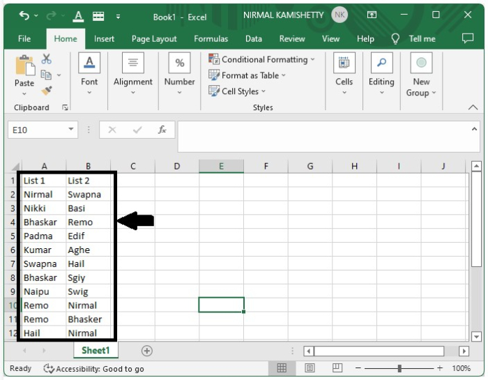
Let us create the list of duplicates names in between the columns. To create an empty column between the two lists, select the second list data and then right-click on the list two and select Insert from the menu box.
From the shown pop-up, select "shift cell to right" and click the "OK" button to create the empty column successfully, as shown in the figure below ?

Step 2
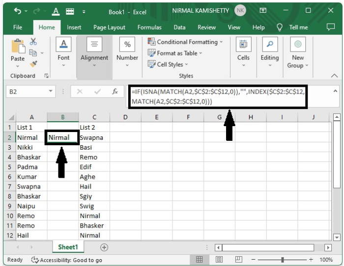
Click the empty cell; in our case, it is the address "B2 cell" and enter the formula as ?
=IF(ISNA(MATCH(A2,$C$2:$C$12,0)),"",INDEX($C$2:$C$12,MATCH(A2,$C$2:$C$12,0)))
and click "Enter" to get the first result as shown in the figure below ?
Step 3
We have successfully created the first result; now to get all the other results, drag down from the right corner of the first result till all the results are filled in Excel. Our final output will look as the screenshot below ?

This is how we can align the duplicates or matching values in two columns in Excel. The only difficulty in this process is the usage of formula; it is very complex.

42K+ Views
