How to compare two columns and delete matches in Excel?

If you want to compare two or more columns to find duplicate values, it can be done using a formula mentioned in this article. Many times, we come across a data set where values are entered repeatedly and required to be filtered. Let’s see how this can be achieved.

Compare Two or More Columns Using a Formula

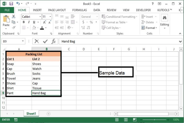
Step 1 − We have taken sample data as shown below having two columns with some duplicate values.

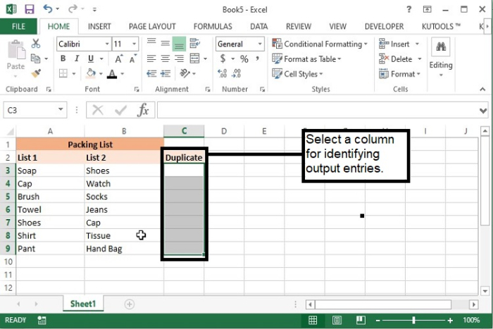
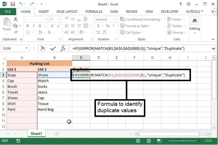
Step 2 − In the column C, we will identify the duplicate and unique values using the below formula.

IF(ISERROR(MATCH(B3,$A$3−$A$10000,0)),"Unique","Duplicate")

Step 3 − Now, in cell C3 enter the above−mentioned formula and drag it to the last row till which data needs to be compared.

Formula Syntax Description

Argument	Description
IF(logical_test, {value_if_true},{value_if_false}	Logical_test specifies the condition basis which the data needs to be rendered. Value_if_true specifies the value that shall be returned if the condition satisfies. Value_if_false specifies the value that shall be returned if the condition does not satisfy.
IsError ( expression )	The IsError function is used to determine if a numeric expression represents an error.
MATCH(lookup_value, lookup_array, [match_type])	lookup_value The value that you want to match in lookup_array. lookup_value argument can be a value or a cell reference to a number, text, or logical value. lookup_array The range of cells being searched. match_type The number −1, 0, or 1. The match_type argument specifies how Excel matches lookup_value with values in lookup_array. The default value for this argument is 1

Step 4 − After dragging the formula till the 9th row, the output will be as follows.

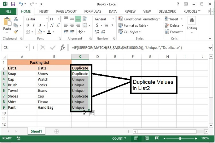
Note − In this sample data, we are comparing List 2 with List 1. Formula will display Duplicate against those records which are available in List 2 as well as List 1.

Delete Duplicate Values

After identifying the duplicate values, they can be deleted at once using the following steps.

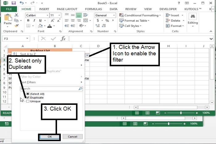
Step 1 − Now, select the column, where duplicate and unique results have been displayed and go to Home tab > Editing Tools > Sort & Filter > Filter.

Step 2 − On click of Filter, a filter will be created in the respective column. Now click the filter arrow and select ‘Duplicate’ option only. Then click OK.

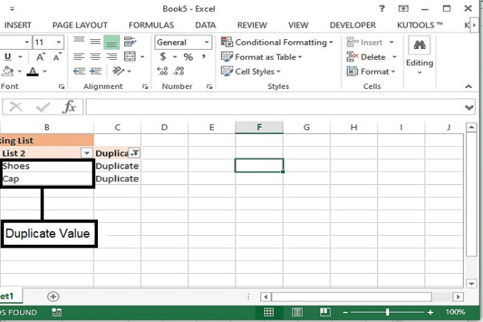
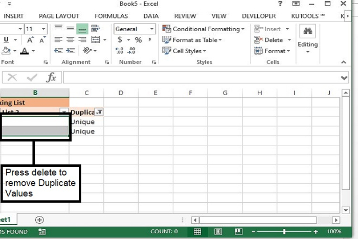
Step 3 − Now it will display only the duplicates, select the values of List2 column, and press Delete key. This will delete the duplicate values available in List2 as compared to the List1.

Step 4 − Now remove the filter and the output will be as following.

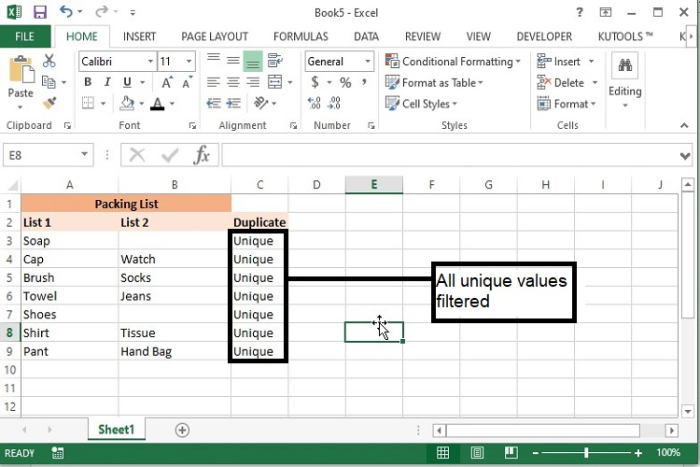
Conclusion

In this way multiple sheets can be compared against 1 sheet and duplicate values can be deleted from all other lists. This method is helpful to get the unique value throughout the data.