
Article Categories
- All Categories
-
 Data Structure
-
 Networking
-
 RDBMS
RDBMS
-
 Operating System
-
 Java
Java
-
 MS Excel
-
 iOS
iOS
-
 HTML
HTML
-
 CSS
CSS
-
 Android
-
 Python
-
 C Programming
-
 C++
C++
-
 C#
C#
-
 MongoDB
-
 MySQL
MySQL
-
 Javascript
-
 PHP
PHP
-
 Economics & Finance
How to compare two columns and return values from the third column in Excel?
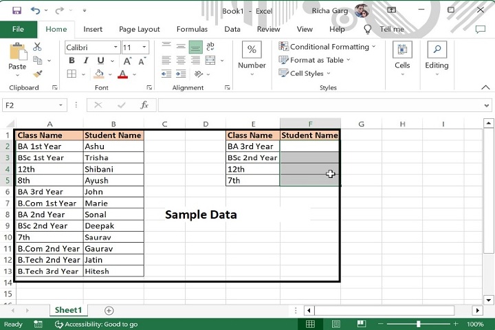
In this article we will learn how to compare values of two columns to get the values from the third column. For example, we have taken a column with Class Names and along with each class name, student name has been written in another column. Now, we will get the students name in another column against some randomly taken class names. Let?s see how this can be achieved using an excel formula.
Compare two columns and getting value from third column with VLOOKUP function
Step 1: We have taken the following sample data for comparison.
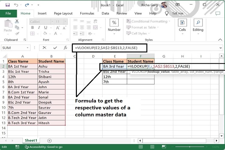
Step 2: Enter the formula in F2 cell as mentioned below. This formula will return names if students as mentioned in column B against the required class names.
=VLOOKUP(E2,$A$2:$B$13,2,FALSE)
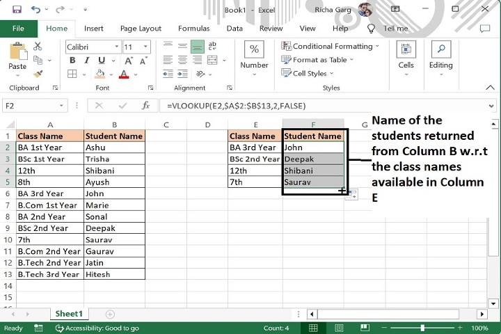
Step 3: Now, drag the formula till the last row of data and the final output will be as following. The formula will display those students names corresponding to the Class name as mentioned in the column E.
| Argument | Description |
|---|---|
| VLOOKUP (lookup_value, table_array, col_index_num, [range_lookup]) |
lookup_value (required) The value you want to look up. The value you want to look up must be in the first column of the range of cells you specify in the table_array argument. table_array (required) The range of cells in which the VLOOKUP will search for the lookup_value and the return value. You can use a named range or a table, and you can use names in the argument instead of cell references. col_index_num (required) The column number (starting with 1 for the left-most column of table_array) that contains the return value. range_lookup (optional) A logical value that specifies whether you want VLOOKUP to find an approximate or an exact match. |
Note
In above formula, E2 is the criteria cell whose value to be find in the master column, A2:A13 is the range of master column in which value of E column to be find, 2 is the index number for column B whose value to be returned and False is to get the exact match of student name.
Conclusion
Hence using the above formula, value of one column can be returned in another column for the identified master set of column one. However, along with this formula there are some more formulas also that can be used for the same purpose like, =INDEX(range of value to get, MATCH(Column 1 to comapre:Column 2 to compare with,0))
7K+ Views
