
Article Categories
- All Categories
-
 Data Structure
-
 Networking
-
 RDBMS
RDBMS
-
 Operating System
-
 Java
Java
-
 MS Excel
-
 iOS
iOS
-
 HTML
HTML
-
 CSS
CSS
-
 Android
-
 Python
-
 C Programming
-
 C++
C++
-
 C#
C#
-
 MongoDB
-
 MySQL
MySQL
-
 Javascript
-
 PHP
PHP
-
 Economics & Finance
How to group adjacent columns or rows separately or independently in Excel?
In this article, learners will understand the process of grouping the adjacent columns in Excel, and its associated benefits. The first and most important benefit of grouping data is that it improves the organization and makes it easier to read and analyze. Users can quickly collapse or expand the group to view the data according to the use and requirement, this will save time and make the spreadsheet professional and more efficient. Another major factor is that it makes the data manipulation easy.
This means that modification and alteration of data become easy. For example, if the user wants to apply formatting or formulas to an entire group of columns at once, rather than having to do it one column at a time and result will appear on all the columns. It also simplifies the process of Data Analysis. In short, while dealing with large data sets, using a group is a very worthy option. Users can collapse those columns that are not required to focus, and similarly, the important data can be expanded to understand the patterns and trends within the provided data. It allows users to enter and process the data effectively. Grouping of column data can be done in a few clicks only. Please refer to the article carefully, to understand the properly.
Example 1: To group adjacent columns or rows separately or independently in Excel by using the predefined available options
Step 1
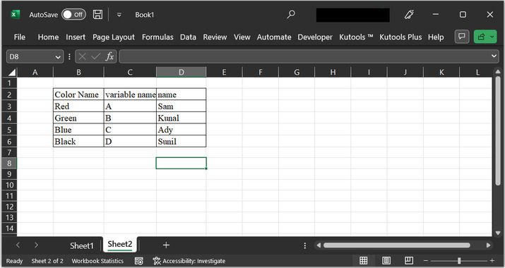
To understand the process of grouping columns or rows separately in Excel, consider the below-given worksheet. This worksheet contains three columns named color name, the variable name, and name. Select the rows or columns the user wants to group. For this example, will select the B column. To select some specific column cell, press the "Ctrl" + arrow (down key) to cover the required number of cells.
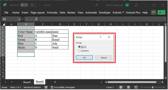
Step 2
After that press shift + "alt"+ right arrow key, to perform the required task. This will display the "group" dialog box. The appears dialog box contains two separate rows for "rows" and "columns" labels.
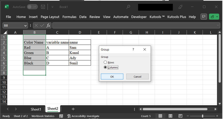
Step 3
In the below given "Group" dialog box, among the provided list of options, click on option "Columns", as here the user wants to group the column data together and finally press the "OK" button. please go through the below-provided image to understand the processing steps properly ?
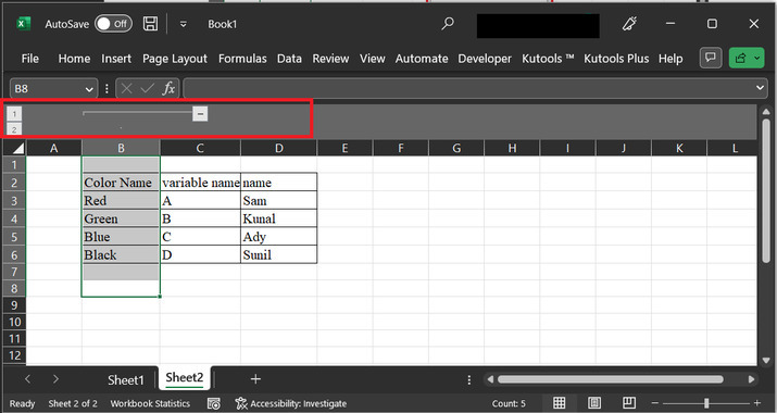
Step 4
Once a grouping is done successfully, the user will be able to see the below-highlighted slider at the bottom of the menu bar. By using the appeared slider, the size of columns can be increased and decreased. If the user drags the column to the right the size of the sheet will increase, but when the column is dragged to leave the data column will be minimized accordingly.
Conclusion
In this article, the user will show the group adjacent columns. So, that the size and other related things can be changed within a single time for multiple columns. The same concept applies to rows as well. Remember in the above-guided steps, will get another option for "rows" inside the group dialog box, by choosing the "rows" option, data can be processed for rows accordingly.

1K+ Views
