
Article Categories
- All Categories
-
 Data Structure
-
 Networking
-
 RDBMS
RDBMS
-
 Operating System
-
 Java
Java
-
 MS Excel
-
 iOS
iOS
-
 HTML
HTML
-
 CSS
CSS
-
 Android
-
 Python
-
 C Programming
-
 C++
C++
-
 C#
C#
-
 MongoDB
-
 MySQL
MySQL
-
 Javascript
-
 PHP
PHP
-
 Economics & Finance
Compare two columns and add missing values in Excel
We all occasionally find ourselves in the position of having to compare columns in Excel. When it comes to comparing and matching data, Microsoft Excel has a lot of alternatives; however, the majority of these options center on searching in a single column. When you have data organized in two distinct columns, you may need to compare them in order to determine which column is lacking certain information and which column contains information that is already there. Depending on what you hope to achieve from making comparisons, you can approach the task in a number of different ways.
Let?s learn how to compare two columns and add missing values through an example.
Using VLOOKUP and ISERROR with IF
Step 1
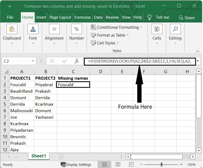
In our example, we have some employee?s name assigned for project1 and project2. We will compare the names of employee for both the projects and add the names who are not present in project 2 in another column. See the following image.

Step 2
Next, we will add another column in that excel sheet and will name it as ?Missing Names?. Then select one blank cell and write the below given formula in formula bar. In our example, we will select C2 and will write the following formula there.
=IF(ISERROR(VLOOKUP(A2,$B$2:$B$12,1,FALSE)),A2,"")
In the above formula,
The acronym VLOOKUP refers to the Vertical Lookup function. VLOOKUP is an Excel function that is already installed on your computer and it allows you to search for a certain value by looking for it vertically across the sheet. That?s why we used VLOOKUP function to compare the data of Project1 with Project2.
The ISERROR function in Excel will return TRUE for every error type that Excel produces, such as #N/A, #VALUE!, #REF!, #DIV/0!, #NUM!, or #NULL!. You can use ISERROR in conjunction with the IF function to check for errors, display a specialized message, or carry out a different calculation depending on whether or not an error was found. In our example, ISERROR function will return the value FALSE if the data is present in both the column, otherwise TRUE.
The IF function performs a logical test and returns one value if the test is TRUE, and a different value if the test is FALSE. In our example, The IF function tells Excel to return the exact name for TRUE and a blank cell for FALSE.
After writing the formula when you press Enter, it will show the name if the name is not present in second column otherwise it will leave the cell blank. See the below given image.
Step 3
To get the formula reflected in other cells, simply click on the ?+? sign appears on the lower-right corner of the cell B2, which activates the autofill function and then drag down. See the below given image.

Conclusion
In this tutorial, we explained how to compare and add the missing name in from both the list using IF, ISERROR and VLOOKUP functions.

3K+ Views
