- Excel Dashboards - Home
- Introduction
- Excel Features Create Dashboards
- Conditional Formatting
- Excel Charts
- Interactive Controls
- Advanced Excel Charts
- Excel PivotTables
- Power PivotTables & PivotCharts
- Power View Reports
- Key Performance Indicators
- Build a Dashboard
- Examples
Excel Dashboards - Conditional Formatting
Conditional Formatting for Data Visualization
If you have chosen Excel for creating dashboard, try to use Excel tables if they serve the purpose. With Conditional Formatting and Sparklines, Excel Tables are the best and simple choice for your dashboard.
In Excel, you can use conditional formatting for data visualization. For example, in a table containing the sales figures for the past quarter region-wise, you can highlight the top 5% values.
You can specify any number of formatting conditions by specifying Rules. You can pick up the Excel built-in Rules that match your conditions from Highlight Cells Rules or Top / Bottom Rules. You can also define your own Rules.
You choose the formatting options that are appropriate for your data visualization - Data Bars, Color Scales, or Icon Sets.
In this chapter, you will learn conditional formatting Rules, formatting options, and adding/managing Rules.
Highlighting Cells
You can use Highlight Cells Rules to assign a format to the cells that contain the data meeting any of the following criteria −
Numbers within a given numerical range: Greater Than, Less Than, Between, and Equal To.
Values that are Duplicate or Unique.
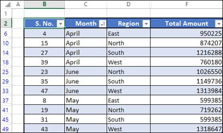
Consider the following summary of results that you want to present −
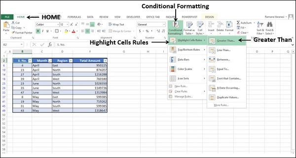
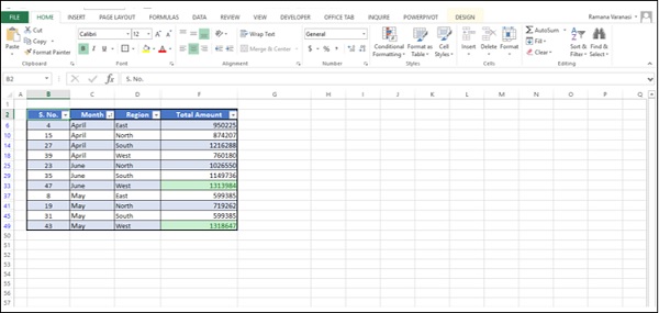
Suppose you want to highlight the Total Amount values that are more than 1000000.
- Select the column Total Amount.
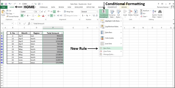
- Click on Conditional Formatting in the Styles group under Home tab.
- Click on Highlight Cells Rules in the dropdown list.
- Click on Greater Than in the second dropdown list that appears.
Greater Than dialog box appears.
In the Format cells that are GREATER THAN: box, specify the condition as 1000000.
In the box with, select the formatting option as Green Fill with Dark Green Text.
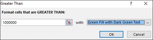
- Click the OK button.
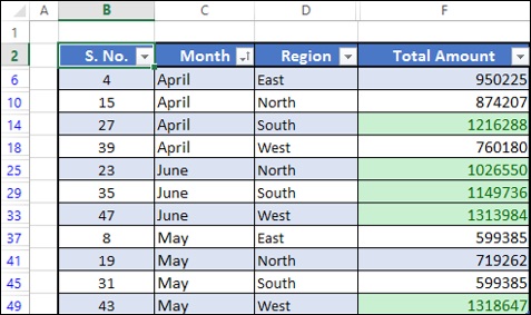
As you can observe, the values satisfying the specified condition are highlighted with the specified format.
Top / Bottom Rules
You can use Top / Bottom Rules to assign a format to the values meeting any of the following criteria −
Top 10 Items − Cells that rank in the top N, where 1 <= N <= 1000.
Top 10% − Cells that rank in the top n%, where 1 <= n <= 100.
Bottom 10 Items − Cells that rank in the bottom N, where 1 <= N <= 1000.
Bottom 10% − Cells that rank in the bottom n%, where 1 <= n <= 100.
Above Average − Cells that are Above Average for the selected range.
Below Average − Cells that are Below Average for the selected range.
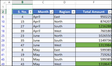
Suppose you want to highlight the Total Amount values that are in top 5%.
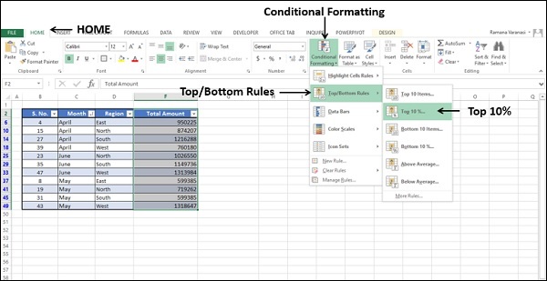
- Select the column Total Amount.
- Click on Conditional Formatting in the Styles group under Home tab.
- Click on Top/Bottom Rules in the dropdown list.
- Click on Top Ten% in the second dropdown list that appears.
Top Ten% dialog box appears.
In the Format cells that rank in the TOP: box, specify the condition as 5%.
In the box with, select the formatting option as Green Fill with Dark Green Text.
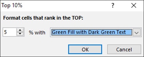
Click the OK button. The top 5% values will be highlighted with the specified format.
Data Bars
You can use colored Data Bars to see the value relative to the other values. The length of the Data Bar represents the value. A longer Bar represents a higher value, and a shorter Bar represents a lower value. You can either use solid colors or gradient colors for Data Bars.
Select the column Total Amount.
Click on Conditional Formatting in the Styles group under Home tab.
Click on Data Bars in the dropdown list.
Click on Blue Data Bar under Gradient Fill in the second dropdown list that appears.
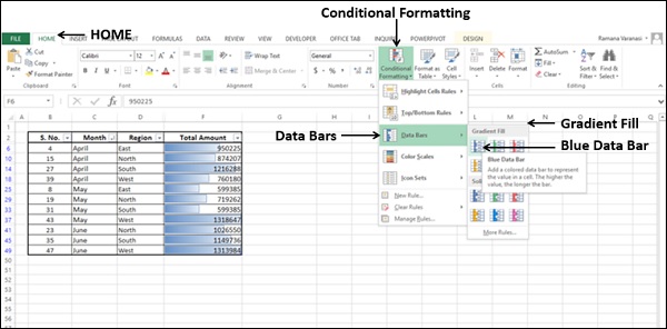
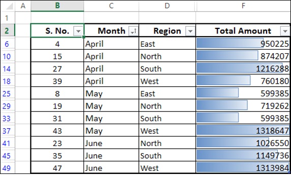
The values in the column will be highlighted showing small, intermediate and large values with blue colored gradient fill bars.
Select the column Total Amount.
Click on Conditional Formatting in the Styles group under Home tab.
Click on Data Bars in the dropdown list.
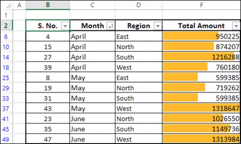
Click on Orange Data Bar under Solid Fill in the second dropdown list that appears.
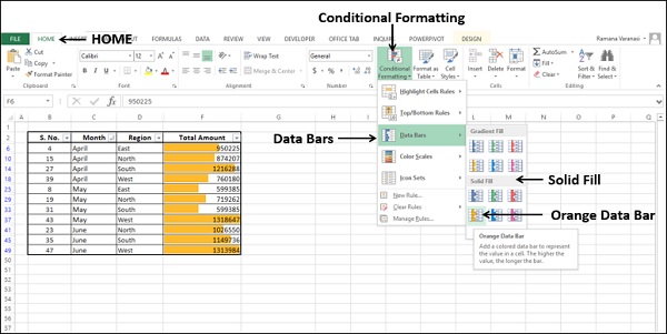
The values in the column will be highlighted showing small, intermediate and large values by bar height with orange colored bars.
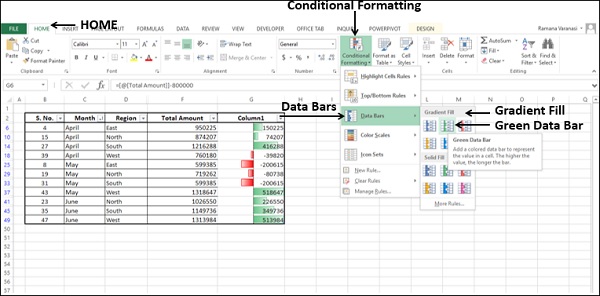
Suppose you want to highlight the sales as compared to a sales target, say 800000.
Create a column with values = [@[Total Amount]]-800000.
Select the new column.
Click on Conditional Formatting in the Styles group under Home tab.
Click on Data Bars in the dropdown list.
Click on Green Data Bar under Gradient Fill in the second dropdown list that appears.
The Data Bars will start in the middle of each cell, and stretch to the left for negative values and to the right for positive values.
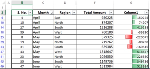
As you can observe, the Bars stretching to the right are green in color indicating positive values and the Bars stretching to the left are red in color indicating negative values.
Color Scales
You can use Color Scales to see the value in a cell relative to the values in the other cells in a column. The color indicates where each cell value falls within that range. You can have either a 3-color scale or 2-color scale.
Select the column Total Amount.
Click on Conditional Formatting in the Styles group under Home tab.
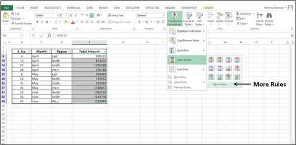
Click on Color Scales in the dropdown list.
Click on Green-Yellow-Red Color Scale in the second dropdown list that appears.
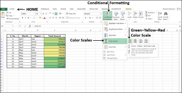
As in the case of Highlight Cells Rules, a Color Scale uses cell shading to display the differences in cell values. As you can observe in the preview, the shade differences are not conspicuous for this data set.
- Click on More Rules in the second dropdown list.
New Formatting Rule dialog box appears.
Click on Format all cells based on their values in the Select a Rule Type box.
In the Edit the Rule Description box, select the following −
Select 3-Color Scale in the Format Style box.
Under Midpoint, for Value type 75.
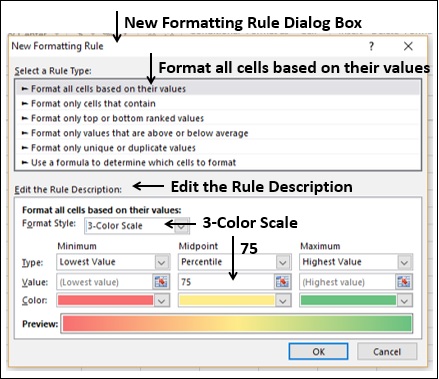
Click the OK button.
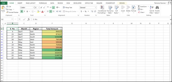
As you can observe, with the defined color scale, the values are distinctly shaded depicting the data range.
Icon Sets
You can use icon sets to visualize numerical differences. In Excel, you have a range of Icon Sets −
| Icon Set Type | Icon Sets |
|---|---|
| Directional | 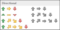 |
| Shapes | 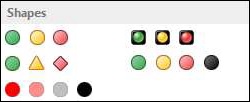 |
| Indicators | 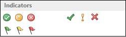 |
| Ratings | 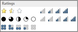 |
As you can observe, an Icon Set consists of three to five symbols. You can define criteria to associate an icon with the values in a cell range. E.g. a red down arrow for small numbers, a green up arrow for large numbers, and a yellow horizontal arrow for intermediate values.
Select the column Total Amount.
Click on Conditional Formatting in the Styles group under Home tab.
Click on Icon Sets in the dropdown list.
Click on 3 Arrows (Colored) in the Directional group in the second dropdown list that appears.
Colored arrows appear in the selected column based on the values.
Using Custom Rules
You can define your own Rules and format a range of cells satisfying a particular condition.
- Select the column Total Amount.
- Click on Conditional Formatting in the Styles group under Home tab.
- Click on New Rule in the dropdown list.
New Formatting Rule dialog box appears.
Click on Use a formula to determine which cells to format, in the Select a Rule Type Box.
In Edit the Rule Description box, do the following −
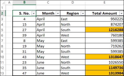
Type a formula in the box - Format values where this formula is true. For example, = PercentRank.INC($E$3:$E$13,E3)>=0.7
Click on Format button.
Choose the format. E.g. Font bold and Fill orange.
Click on OK.
Check the Preview.
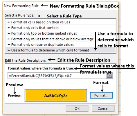
Click on OK if the Preview is alright. The values in the data set that are satisfying the formula will be highlighted with the format you have chosen.
Managing Conditional Formatting Rules
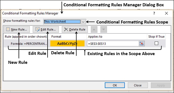
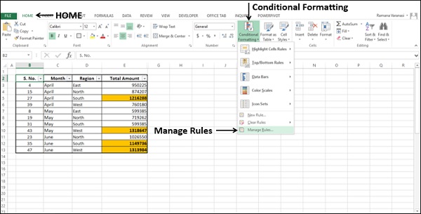
You can manage the conditional formatting Rules using the Conditional Formatting Rules Manager dialog box.
Click Conditional Formatting in the Styles group under Home tab. Click Manage Rules in the dropdown list.
Conditional Formatting Rules Manager dialog box appears. You can view all the existing Rules. You can add a new Rule, delete a Rule and/or edit a Rule to modify it.