- DSA - Home
- DSA - Overview
- DSA - Environment Setup
- DSA - Algorithms Basics
- DSA - Asymptotic Analysis
- Data Structures
- DSA - Data Structure Basics
- DSA - Data Structures and Types
- DSA - Array Data Structure
- DSA - Skip List Data Structure
- Linked Lists
- DSA - Linked List Data Structure
- DSA - Doubly Linked List Data Structure
- DSA - Circular Linked List Data Structure
- Stack & Queue
- DSA - Stack Data Structure
- DSA - Expression Parsing
- DSA - Queue Data Structure
- DSA - Circular Queue Data Structure
- DSA - Priority Queue Data Structure
- DSA - Deque Data Structure
- Searching Algorithms
- DSA - Searching Algorithms
- DSA - Linear Search Algorithm
- DSA - Binary Search Algorithm
- DSA - Interpolation Search
- DSA - Jump Search Algorithm
- DSA - Exponential Search
- DSA - Fibonacci Search
- DSA - Sublist Search
- DSA - Hash Table
- Sorting Algorithms
- DSA - Sorting Algorithms
- DSA - Bubble Sort Algorithm
- DSA - Insertion Sort Algorithm
- DSA - Selection Sort Algorithm
- DSA - Merge Sort Algorithm
- DSA - Shell Sort Algorithm
- DSA - Heap Sort Algorithm
- DSA - Bucket Sort Algorithm
- DSA - Counting Sort Algorithm
- DSA - Radix Sort Algorithm
- DSA - Quick Sort Algorithm
- Matrices Data Structure
- DSA - Matrices Data Structure
- DSA - Lup Decomposition In Matrices
- DSA - Lu Decomposition In Matrices
- Graph Data Structure
- DSA - Graph Data Structure
- DSA - Depth First Traversal
- DSA - Breadth First Traversal
- DSA - Spanning Tree
- DSA - Topological Sorting
- DSA - Strongly Connected Components
- DSA - Biconnected Components
- DSA - Augmenting Path
- DSA - Network Flow Problems
- DSA - Flow Networks In Data Structures
- DSA - Edmonds Blossom Algorithm
- DSA - Maxflow Mincut Theorem
- Tree Data Structure
- DSA - Tree Data Structure
- DSA - Tree Traversal
- DSA - Binary Search Tree
- DSA - AVL Tree
- DSA - Red Black Trees
- DSA - B Trees
- DSA - B+ Trees
- DSA - Splay Trees
- DSA - Range Queries
- DSA - Segment Trees
- DSA - Fenwick Tree
- DSA - Fusion Tree
- DSA - Hashed Array Tree
- DSA - K-Ary Tree
- DSA - Kd Trees
- DSA - Priority Search Tree Data Structure
- Recursion
- DSA - Recursion Algorithms
- DSA - Tower of Hanoi Using Recursion
- DSA - Fibonacci Series Using Recursion
- Divide and Conquer
- DSA - Divide and Conquer
- DSA - Max-Min Problem
- DSA - Strassen's Matrix Multiplication
- DSA - Karatsuba Algorithm
- Greedy Algorithms
- DSA - Greedy Algorithms
- DSA - Travelling Salesman Problem (Greedy Approach)
- DSA - Prim's Minimal Spanning Tree
- DSA - Kruskal's Minimal Spanning Tree
- DSA - Dijkstra's Shortest Path Algorithm
- DSA - Map Colouring Algorithm
- DSA - Fractional Knapsack Problem
- DSA - Job Sequencing with Deadline
- DSA - Optimal Merge Pattern Algorithm
- Dynamic Programming
- DSA - Dynamic Programming
- DSA - Matrix Chain Multiplication
- DSA - Floyd Warshall Algorithm
- DSA - 0-1 Knapsack Problem
- DSA - Longest Common Sub-sequence Algorithm
- DSA - Travelling Salesman Problem (Dynamic Approach)
- Hashing
- DSA - Hashing Data Structure
- DSA - Collision In Hashing
- Disjoint Set
- DSA - Disjoint Set
- DSA - Path Compression And Union By Rank
- Heap
- DSA - Heap Data Structure
- DSA - Binary Heap
- DSA - Binomial Heap
- DSA - Fibonacci Heap
- Tries Data Structure
- DSA - Tries
- DSA - Standard Tries
- DSA - Compressed Tries
- DSA - Suffix Tries
- Treaps
- DSA - Treaps Data Structure
- Bit Mask
- DSA - Bit Mask In Data Structures
- Bloom Filter
- DSA - Bloom Filter Data Structure
- Approximation Algorithms
- DSA - Approximation Algorithms
- DSA - Vertex Cover Algorithm
- DSA - Set Cover Problem
- DSA - Travelling Salesman Problem (Approximation Approach)
- Randomized Algorithms
- DSA - Randomized Algorithms
- DSA - Randomized Quick Sort Algorithm
- DSA - Karger’s Minimum Cut Algorithm
- DSA - Fisher-Yates Shuffle Algorithm
- Miscellaneous
- DSA - Infix to Postfix
- DSA - Bellmon Ford Shortest Path
- DSA - Maximum Bipartite Matching
- DSA Useful Resources
- DSA - Questions and Answers
- DSA - Selection Sort Interview Questions
- DSA - Merge Sort Interview Questions
- DSA - Insertion Sort Interview Questions
- DSA - Heap Sort Interview Questions
- DSA - Bubble Sort Interview Questions
- DSA - Bucket Sort Interview Questions
- DSA - Radix Sort Interview Questions
- DSA - Cycle Sort Interview Questions
- DSA - Quick Guide
- DSA - Useful Resources
- DSA - Discussion
Data Structures - Algorithms Basics

Algorithm is a step-by-step procedure, which defines a set of instructions to be executed in a certain order to get the desired output. Algorithms are generally created independent of underlying languages, i.e. an algorithm can be implemented in more than one programming language.
From the data structure point of view, following are some important categories of algorithms −
Search − Algorithm to search an item in a data structure.
Sort − Algorithm to sort items in a certain order.
Insert − Algorithm to insert item in a data structure.
Update − Algorithm to update an existing item in a data structure.
Delete − Algorithm to delete an existing item from a data structure.
Characteristics of an Algorithm
Not all procedures can be called an algorithm. An algorithm should have the following characteristics −
Unambiguous − Algorithm should be clear and unambiguous. Each of its steps (or phases), and their inputs/outputs should be clear and must lead to only one meaning.
Input − An algorithm should have 0 or more well-defined inputs.
Output − An algorithm should have 1 or more well-defined outputs, and should match the desired output.
Finiteness − Algorithms must terminate after a finite number of steps.
Feasibility − Should be feasible with the available resources.
Independent − An algorithm should have step-by-step directions, which should be independent of any programming code.
How to Write an Algorithm?
There are no well-defined standards for writing algorithms. Rather, it is problem and resource dependent. Algorithms are never written to support a particular programming code.
As we know that all programming languages share basic code constructs like loops (do, for, while), flow-control (if-else), etc. These common constructs can be used to write an algorithm.
We write algorithms in a step-by-step manner, but it is not always the case. Algorithm writing is a process and is executed after the problem domain is well-defined. That is, we should know the problem domain, for which we are designing a solution.
Example
Let's try to learn algorithm-writing by using an example.
Problem − Design an algorithm to add two numbers and display the result.
Step 1 − START
Step 2 − declare three integers a, b & c
Step 3 − define values of a & b
Step 4 − add values of a & b
Step 5 − store output of step 4 to c
Step 6 − print c
Step 7 − STOP
Algorithms tell the programmers how to code the program. Alternatively, the algorithm can be written as −
Step 1 − START ADD
Step 2 − get values of a & b
Step 3 − c ← a + b
Step 4 − display c
Step 5 − STOP
In design and analysis of algorithms, usually the second method is used to describe an algorithm. It makes it easy for the analyst to analyze the algorithm ignoring all unwanted definitions. He can observe what operations are being used and how the process is flowing.
Writing step numbers, is optional.
We design an algorithm to get a solution of a given problem. A problem can be solved in more than one ways.
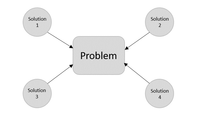
Hence, many solution algorithms can be derived for a given problem. The next step is to analyze those proposed solution algorithms and implement the best suitable solution.
Algorithm Analysis
Efficiency of an algorithm can be analyzed at two different stages, before implementation and after implementation. They are the following −
A Priori Analysis − This is a theoretical analysis of an algorithm. Efficiency of an algorithm is measured by assuming that all other factors, for example, processor speed, are constant and have no effect on the implementation.
A Posterior Analysis − This is an empirical analysis of an algorithm. The selected algorithm is implemented using programming language. This is then executed on target computer machine. In this analysis, actual statistics like running time and space required, are collected.
We shall learn about a priori algorithm analysis. Algorithm analysis deals with the execution or running time of various operations involved. The running time of an operation can be defined as the number of computer instructions executed per operation.
Algorithm Complexity
Suppose X is an algorithm and n is the size of input data, the time and space used by the algorithm X are the two main factors, which decide the efficiency of X.
Time Factor − Time is measured by counting the number of key operations such as comparisons in the sorting algorithm.
Space Factor − Space is measured by counting the maximum memory space required by the algorithm.
The complexity of an algorithm f(n) gives the running time and/or the storage space required by the algorithm in terms of n as the size of input data.
Space Complexity
Space complexity of an algorithm represents the amount of memory space required by the algorithm in its life cycle. The space required by an algorithm is equal to the sum of the following two components −
A fixed part that is a space required to store certain data and variables, that are independent of the size of the problem. For example, simple variables and constants used, program size, etc.
A variable part is a space required by variables, whose size depends on the size of the problem. For example, dynamic memory allocation, recursion stack space, etc.
Space complexity S(P) of any algorithm P is S(P) = C + SP(I), where C is the fixed part and S(I) is the variable part of the algorithm, which depends on instance characteristic I. Following is a simple example that tries to explain the concept −
Algorithm: SUM(A, B)
Step 1 − START
Step 2 − C ← A + B + 10
Step 3 − Stop
Here we have three variables A, B, and C and one constant. Hence S(P) = 1 + 3. Now, space depends on data types of given variables and constant types and it will be multiplied accordingly.
Time Complexity
Time complexity of an algorithm represents the amount of time required by the algorithm to run to completion. Time requirements can be defined as a numerical function T(n), where T(n) can be measured as the number of steps, provided each step consumes constant time.
For example, addition of two n-bit integers takes n steps. Consequently, the total computational time is T(n) = c ∗ n, where c is the time taken for the addition of two bits. Here, we observe that T(n) grows linearly as the input size increases.
