
Article Categories
- All Categories
-
 Data Structure
-
 Networking
-
 RDBMS
RDBMS
-
 Operating System
-
 Java
Java
-
 MS Excel
-
 iOS
iOS
-
 HTML
HTML
-
 CSS
CSS
-
 Android
-
 Python
-
 C Programming
-
 C++
C++
-
 C#
C#
-
 MongoDB
-
 MySQL
MySQL
-
 Javascript
-
 PHP
PHP
-
 Economics & Finance
What is the performance measure of branch processing in computer architecture?
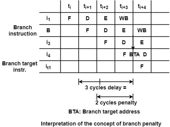
It can evaluate and compare different branch processing techniques, it can require a performance measure. Let us consider the execution of a branch instruction in a four-stage pipeline as shown in the figure. If the branch is processed straightforwardly, the branch target address (BTA) will be computed in cycle ti+3.
Then the branch target instruction can be fetched in cycle ti+4. Thus, the branch target instruction is fetched with a 3 cycles delay in comparison to the fetching of the branch instruction. This means a 2-cycle penalty compared to the sequential processing.
The performance of branch processing in a certain typical situation. Let us denote the penalties of ‘taken’ and ‘not taken’ branches by Ptand Pnt and the corresponding probabilities (frequencies) of ‘taken’ and ‘not taken’ branches as ftand fnt. Then the effective penalty of branch processing P is
P = f<sub>t</sub> ∗ P<sub>t</sub>+ f<sub>nt</sub> ∗ P<sub>nt</sub>
For example, it can calculate the effective penalties of the 80386 and i486 processors. For the 80386 the values of the taken and not-taken penalties are 8 and 2 cycles, respectively. When the probability of taken branches is assumed to be 0.75 (fi=0.75), it can get the effective penalty of branches in the 80386 −
P<sub>80386</sub>=0.75 ∗ 8+0.25 ∗ 2=6.5 cycles
This means that the 80386 requires, on average, 6.5 additional cycles for each branch. In contrast, the i486 has a substantially enhanced branch mechanism. Its effective branch penalty is
P<sub>i486</sub>=0.75 ∗ 2+0.25 ∗ 0=1.5
Which is considerably less than the penalty of 80386.
A further typical situation is when branch processing uses branch prediction. In this case, a prediction is made for each branch by guessing whether the branch in question will be taken or not. Let us consider the following notation −
Ptc − penalty for correctly predicted taken branches
Ptm − penalty for mispredicted taken branches
Pntc − penalty for correctly predicted not-taken branches
Pntm − penalty for mispredicted not-taken branches
ftc − probability for correctly predicted taken branches
ftm − probability for mispredicted taken branches
fntc − probability for correctly predicted not-taken branches
fntm − probability for mispredicted not-taken branches
Then, the effective penalty of branch processing can be expressed as −
P=f<sub>tc</sub>∗P<sub>tc</sub>+f<sub>tm</sub>∗P<sub>tm</sub>+f<sub>ntc</sub>∗P<sub>ntc</sub>+f<sub>ntm</sub>∗Pntm
It can assume a straightforward case when the branch penalties for correctly predicted taken and not-taken branches, and for mispredicted taken and not-taken branches are equal. That is
P<sub>tc</sub>=P<sub>ntc</sub>and P<sub>tm</sub>=P<sub>ntm</sub>
Furthermore, let us designate the total probability of correctly predicted branches as fc and that of mispredicted branches as fm, that is
f<sub>c</sub>=f<sub>tc</sub>+f<sub>ntc</sub>and f<sub>m</sub>=f<sub>tm</sub>+f<sub>ntm</sub>
In this straightforward case, the effective branch penalty can be calculated as
P=f<sub>c</sub>∗P<sub>c</sub>+f<sub>m</sub>∗P<sub>m</sub>
Let us consider the Pentium processor which uses branch prediction. In this case, the penalty for correctly predicted branches is 0 cycles, whereas that for mispredicted branches equals wither 3 cycles (if the branch is processed by the U pipe) or 4 cycles (if the branch is executed in the V pipe).
For the calculation, let us suppose an average misprediction penalty of 3.5. When it assumes a branch prediction accuracy of 0.9 (that is, fc=0.9 and fm=0.1) we get the effective branch penalty of this processor
P<sub>Pentium</sub>=0.9∗0+0.1∗3.5=0.35
That is Pentium requires, on average, only 0.35 additional cycles for branches.

740 Views
