- Time Series - Home
- Time Series - Introduction
- Time Series - Programming Languages
- Time Series - Python Libraries
- Data Processing & Visualization
- Time Series - Modeling
- Time Series - Parameter Calibration
- Time Series - Naive Methods
- Time Series - Auto Regression
- Time Series - Moving Average
- Time Series - ARIMA
- Time Series - Variations of ARIMA
- Time Series - Exponential Smoothing
- Time Series - Walk Forward Validation
- Time Series - Prophet Model
- Time Series - LSTM Model
- Time Series - Error Metrics
- Time Series - Applications
- Time Series - Further Scope
- Time Series Useful Resources
- Time Series - Quick Guide
- Time Series - Useful Resources
- Time Series - Discussion
Time Series - Variations of ARIMA
In the previous chapter, we have now seen how ARIMA model works, and its limitations that it cannot handle seasonal data or multivariate time series and hence, new models were introduced to include these features.
A glimpse of these new models is given here −
Vector Auto-Regression (VAR)
It is a generalized version of auto regression model for multivariate stationary time series. It is characterized by p parameter.
Vector Moving Average (VMA)
It is a generalized version of moving average model for multivariate stationary time series. It is characterized by q parameter.
Vector Auto Regression Moving Average (VARMA)
It is the combination of VAR and VMA and a generalized version of ARMA model for multivariate stationary time series. It is characterized by p and q parameters. Much like, ARMA is capable of acting like an AR model by setting q parameter as 0 and as a MA model by setting p parameter as 0, VARMA is also capable of acting like an VAR model by setting q parameter as 0 and as a VMA model by setting p parameter as 0.
In [209]:
df_multi = df[['T', 'C6H6(GT)']]
split = len(df) - int(0.2*len(df))
train_multi, test_multi = df_multi[0:split], df_multi[split:]
In [211]:
from statsmodels.tsa.statespace.varmax import VARMAX

model = VARMAX(train_multi, order = (2,1))
model_fit = model.fit()
c:\users\naveksha\appdata\local\programs\python\python37\lib\site-packages\statsmodels\tsa\statespace\varmax.py:152:
   EstimationWarning: Estimation of VARMA(p,q) models is not generically robust,
   due especially to identification issues.
   EstimationWarning)
c:\users\naveksha\appdata\local\programs\python\python37\lib\site-packages\statsmodels\tsa\base\tsa_model.py:171:
   ValueWarning: No frequency information was provided, so inferred frequency H will be used.
  % freq, ValueWarning)
c:\users\naveksha\appdata\local\programs\python\python37\lib\site-packages\statsmodels\base\model.py:508:
   ConvergenceWarning: Maximum Likelihood optimization failed to converge. Check mle_retvals
  "Check mle_retvals", ConvergenceWarning)
In [213]:
predictions_multi = model_fit.forecast( steps=len(test_multi))
c:\users\naveksha\appdata\local\programs\python\python37\lib\site-packages\statsmodels\tsa\base\tsa_model.py:320:
   FutureWarning: Creating a DatetimeIndex by passing range endpoints is deprecated.  Use `pandas.date_range` instead.
   freq = base_index.freq)
c:\users\naveksha\appdata\local\programs\python\python37\lib\site-packages\statsmodels\tsa\statespace\varmax.py:152:
   EstimationWarning: Estimation of VARMA(p,q) models is not generically robust, due especially to identification issues.
   EstimationWarning)
In [231]:
plt.plot(train_multi['T'])
plt.plot(test_multi['T'])
plt.plot(predictions_multi.iloc[:,0:1], '--')
plt.show()

plt.plot(train_multi['C6H6(GT)'])
plt.plot(test_multi['C6H6(GT)'])
plt.plot(predictions_multi.iloc[:,1:2], '--')
plt.show()
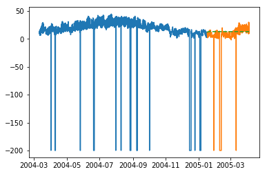
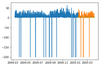
The above code shows how VARMA model can be used to model multivariate time series, although this model may not be best suited on our data.
VARMA with Exogenous Variables (VARMAX)
It is an extension of VARMA model where extra variables called covariates are used to model the primary variable we are interested it.
Seasonal Auto Regressive Integrated Moving Average (SARIMA)
This is the extension of ARIMA model to deal with seasonal data. It divides the data into seasonal and non-seasonal components and models them in a similar fashion. It is characterized by 7 parameters, for non-seasonal part (p,d,q) parameters same as for ARIMA model and for seasonal part (P,D,Q,m) parameters where m is the number of seasonal periods and P,D,Q are similar to parameters of ARIMA model. These parameters can be calibrated using grid search or genetic algorithm.
SARIMA with Exogenous Variables (SARIMAX)
This is the extension of SARIMA model to include exogenous variables which help us to model the variable we are interested in.
It may be useful to do a co-relation analysis on variables before putting them as exogenous variables.
In [251]:
from scipy.stats.stats import pearsonr
x = train_multi['T'].values
y = train_multi['C6H6(GT)'].values

corr , p = pearsonr(x,y)
print ('Corelation Coefficient =', corr,'\nP-Value =',p)
Corelation Coefficient = 0.9701173437269858
P-Value = 0.0
Pearsons Correlation shows a linear relation between 2 variables, to interpret the results, we first look at the p-value, if it is less that 0.05 then the value of coefficient is significant, else the value of coefficient is not significant. For significant p-value, a positive value of correlation coefficient indicates positive correlation, and a negative value indicates a negative correlation.
Hence, for our data, temperature and C6H6 seem to have a highly positive correlation. Therefore, we will
In [297]:
from statsmodels.tsa.statespace.sarimax import SARIMAX

model = SARIMAX(x, exog = y, order = (2, 0, 2), seasonal_order = (2, 0, 1, 1), enforce_stationarity=False, enforce_invertibility = False)
model_fit = model.fit(disp = False)
c:\users\naveksha\appdata\local\programs\python\python37\lib\site-packages\statsmodels\base\model.py:508:
   ConvergenceWarning: Maximum Likelihood optimization failed to converge. Check mle_retvals
   "Check mle_retvals", ConvergenceWarning)
In [298]:
y_ = test_multi['C6H6(GT)'].values
predicted = model_fit.predict(exog=y_)
test_multi_ = pandas.DataFrame(test)
test_multi_['predictions'] = predicted[0:1871]
In [299]:
plt.plot(train_multi['T'])
plt.plot(test_multi_['T'])
plt.plot(test_multi_.predictions, '--')
Out[299]:
[<matplotlib.lines.Line2D at 0x1eab0191c18>]
The predictions here seem to take larger variations now as opposed to univariate ARIMA modelling.
Needless to say, SARIMAX can be used as an ARX, MAX, ARMAX or ARIMAX model by setting only the corresponding parameters to non-zero values.
Fractional Auto Regressive Integrated Moving Average (FARIMA)
At times, it may happen that our series is not stationary, yet differencing with d parameter taking the value 1 may over-difference it. So, we need to difference the time series using a fractional value.
In the world of data science there is no one superior model, the model that works on your data depends greatly on your dataset. Knowledge of various models allows us to choose one that work on our data and experimenting with that model to achieve the best results. And results should be seen as plot as well as error metrics, at times a small error may also be bad, hence, plotting and visualizing the results is essential.
In the next chapter, we will be looking at another statistical model, exponential smoothing.
