- Time Series - Home
- Time Series - Introduction
- Time Series - Programming Languages
- Time Series - Python Libraries
- Data Processing & Visualization
- Time Series - Modeling
- Time Series - Parameter Calibration
- Time Series - Naive Methods
- Time Series - Auto Regression
- Time Series - Moving Average
- Time Series - ARIMA
- Time Series - Variations of ARIMA
- Time Series - Exponential Smoothing
- Time Series - Walk Forward Validation
- Time Series - Prophet Model
- Time Series - LSTM Model
- Time Series - Error Metrics
- Time Series - Applications
- Time Series - Further Scope
- Time Series Useful Resources
- Time Series - Quick Guide
- Time Series - Useful Resources
- Time Series - Discussion
Time Series - Exponential Smoothing
In this chapter, we will talk about the techniques involved in exponential smoothing of time series.
Simple Exponential Smoothing
Exponential Smoothing is a technique for smoothing univariate time-series by assigning exponentially decreasing weights to data over a time period.
Mathematically, the value of variable at time t+1 given value at time t, y_(t+1|t) is defined as −
$$y_{t+1|t}\:=\:\alpha y_{t}\:+\:\alpha\lgroup1 -\alpha\rgroup y_{t-1}\:+\alpha\lgroup1-\alpha\rgroup^{2}\:y_{t-2}\:+\:...+y_{1}$$
where,$0\leq\alpha \leq1$ is the smoothing parameter, and
$y_{1},....,y_{t}$ are previous values of network traffic at times 1, 2, 3, ,t.
This is a simple method to model a time series with no clear trend or seasonality. But exponential smoothing can also be used for time series with trend and seasonality.
Triple Exponential Smoothing
Triple Exponential Smoothing (TES) or Holt's Winter method, applies exponential smoothing three times - level smoothing $l_{t}$, trend smoothing $b_{t}$, and seasonal smoothing $S_{t}$, with $\alpha$, $\beta^{*}$ and $\gamma$ as smoothing parameters with m as the frequency of the seasonality, i.e. the number of seasons in a year.
According to the nature of the seasonal component, TES has two categories −
Holt-Winter's Additive Method − When the seasonality is additive in nature.
Holt-Winters Multiplicative Method − When the seasonality is multiplicative in nature.
For non-seasonal time series, we only have trend smoothing and level smoothing, which is called Holts Linear Trend Method.
Lets try applying triple exponential smoothing on our data.
In [316]:
from statsmodels.tsa.holtwinters import ExponentialSmoothing

model = ExponentialSmoothing(train.values, trend= )
model_fit = model.fit()
In [322]:
predictions_ = model_fit.predict(len(test))
In [325]:
plt.plot(test.values)
plt.plot(predictions_[1:1871])
Out[325]:
[<matplotlib.lines.Line2D at 0x1eab00f1cf8>]
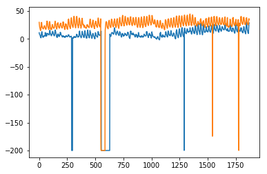
Here, we have trained the model once with training set and then we keep on making predictions. A more realistic approach is to re-train the model after one or more time step(s). As we get the prediction for time t+1 from training data til time t, the next prediction for time t+2 can be made using the training data til time t+1 as the actual value at t+1 will be known then. This methodology of making predictions for one or more future steps and then re-training the model is called rolling forecast or walk forward validation.
