- Time Series - Home
- Time Series - Introduction
- Time Series - Programming Languages
- Time Series - Python Libraries
- Data Processing & Visualization
- Time Series - Modeling
- Time Series - Parameter Calibration
- Time Series - Naive Methods
- Time Series - Auto Regression
- Time Series - Moving Average
- Time Series - ARIMA
- Time Series - Variations of ARIMA
- Time Series - Exponential Smoothing
- Time Series - Walk Forward Validation
- Time Series - Prophet Model
- Time Series - LSTM Model
- Time Series - Error Metrics
- Time Series - Applications
- Time Series - Further Scope
- Time Series Useful Resources
- Time Series - Quick Guide
- Time Series - Useful Resources
- Time Series - Discussion
Time Series - LSTM Model
Now, we are familiar with statistical modelling on time series, but machine learning is all the rage right now, so it is essential to be familiar with some machine learning models as well. We shall start with the most popular model in time series domain − Long Short-term Memory model.
LSTM is a class of recurrent neural network. So before we can jump to LSTM, it is essential to understand neural networks and recurrent neural networks.
Neural Networks
An artificial neural network is a layered structure of connected neurons, inspired by biological neural networks. It is not one algorithm but combinations of various algorithms which allows us to do complex operations on data.
Recurrent Neural Networks
It is a class of neural networks tailored to deal with temporal data. The neurons of RNN have a cell state/memory, and input is processed according to this internal state, which is achieved with the help of loops with in the neural network. There are recurring module(s) of tanh layers in RNNs that allow them to retain information. However, not for a long time, which is why we need LSTM models.
LSTM
It is special kind of recurrent neural network that is capable of learning long term dependencies in data. This is achieved because the recurring module of the model has a combination of four layers interacting with each other.
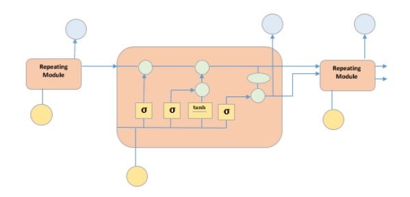
The picture above depicts four neural network layers in yellow boxes, point wise operators in green circles, input in yellow circles and cell state in blue circles. An LSTM module has a cell state and three gates which provides them with the power to selectively learn, unlearn or retain information from each of the units. The cell state in LSTM helps the information to flow through the units without being altered by allowing only a few linear interactions. Each unit has an input, output and a forget gate which can add or remove the information to the cell state. The forget gate decides which information from the previous cell state should be forgotten for which it uses a sigmoid function. The input gate controls the information flow to the current cell state using a point-wise multiplication operation of sigmoid and tanh respectively. Finally, the output gate decides which information should be passed on to the next hidden state
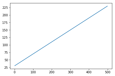
Now that we have understood the internal working of LSTM model, let us implement it. To understand the implementation of LSTM, we will start with a simple example − a straight line. Let us see, if LSTM can learn the relationship of a straight line and predict it.
First let us create the dataset depicting a straight line.
In [402]:
x = numpy.arange (1,500,1)
y = 0.4 * x + 30
plt.plot(x,y)
Out[402]:
[<matplotlib.lines.Line2D at 0x1eab9d3ee10>]
In [403]:
trainx, testx = x[0:int(0.8*(len(x)))], x[int(0.8*(len(x))):]
trainy, testy = y[0:int(0.8*(len(y)))], y[int(0.8*(len(y))):]
train = numpy.array(list(zip(trainx,trainy)))
test = numpy.array(list(zip(trainx,trainy)))
Now that the data has been created and split into train and test. Lets convert the time series data into the form of supervised learning data according to the value of look-back period, which is essentially the number of lags which are seen to predict the value at time t.
So a time series like this −
time variable_x
t1  x1
t2  x2
 :   :
 :   :
T   xT
When look-back period is 1, is converted to −
x1   x2
x2   x3
 :    :
 :    :
xT-1 xT
In [404]:
def create_dataset(n_X, look_back):
   dataX, dataY = [], []
   for i in range(len(n_X)-look_back):
      a = n_X[i:(i+look_back), ]
      dataX.append(a)
      dataY.append(n_X[i + look_back, ])
   return numpy.array(dataX), numpy.array(dataY)
In [405]:
look_back = 1
trainx,trainy = create_dataset(train, look_back)
testx,testy = create_dataset(test, look_back)

trainx = numpy.reshape(trainx, (trainx.shape[0], 1, 2))
testx = numpy.reshape(testx, (testx.shape[0], 1, 2))
Now we will train our model.
Small batches of training data are shown to network, one run of when entire training data is shown to the model in batches and error is calculated is called an epoch. The epochs are to be run til the time the error is reducing.
In [ ]:
from keras.models import Sequential
from keras.layers import LSTM, Dense

model = Sequential()
model.add(LSTM(256, return_sequences = True, input_shape = (trainx.shape[1], 2)))
model.add(LSTM(128,input_shape = (trainx.shape[1], 2)))
model.add(Dense(2))
model.compile(loss = 'mean_squared_error', optimizer = 'adam')
model.fit(trainx, trainy, epochs = 2000, batch_size = 10, verbose = 2, shuffle = False)
model.save_weights('LSTMBasic1.h5')
In [407]:
model.load_weights('LSTMBasic1.h5')
predict = model.predict(testx)
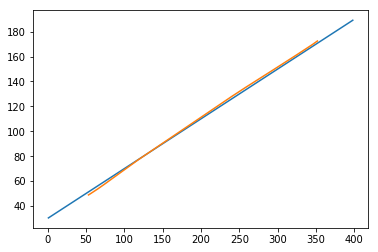
Now lets see what our predictions look like.
In [408]:
plt.plot(testx.reshape(398,2)[:,0:1], testx.reshape(398,2)[:,1:2])
plt.plot(predict[:,0:1], predict[:,1:2])
Out[408]:
[<matplotlib.lines.Line2D at 0x1eac792f048>]
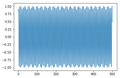
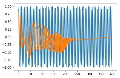
Now, we should try and model a sine or cosine wave in a similar fashion. You can run the code given below and play with the model parameters to see how the results change.
In [409]:
x = numpy.arange (1,500,1)
y = numpy.sin(x)
plt.plot(x,y)
Out[409]:
[<matplotlib.lines.Line2D at 0x1eac7a0b3c8>]
In [410]:
trainx, testx = x[0:int(0.8*(len(x)))], x[int(0.8*(len(x))):]
trainy, testy = y[0:int(0.8*(len(y)))], y[int(0.8*(len(y))):]
train = numpy.array(list(zip(trainx,trainy)))
test = numpy.array(list(zip(trainx,trainy)))
In [411]:
look_back = 1
trainx,trainy = create_dataset(train, look_back)
testx,testy = create_dataset(test, look_back)
trainx = numpy.reshape(trainx, (trainx.shape[0], 1, 2))
testx = numpy.reshape(testx, (testx.shape[0], 1, 2))
In [ ]:
model = Sequential()
model.add(LSTM(512, return_sequences = True, input_shape = (trainx.shape[1], 2)))
model.add(LSTM(256,input_shape = (trainx.shape[1], 2)))
model.add(Dense(2))
model.compile(loss = 'mean_squared_error', optimizer = 'adam')
model.fit(trainx, trainy, epochs = 2000, batch_size = 10, verbose = 2, shuffle = False)
model.save_weights('LSTMBasic2.h5')
In [413]:
model.load_weights('LSTMBasic2.h5')
predict = model.predict(testx)
In [415]:
plt.plot(trainx.reshape(398,2)[:,0:1], trainx.reshape(398,2)[:,1:2])
plt.plot(predict[:,0:1], predict[:,1:2])
Out [415]:
[<matplotlib.lines.Line2D at 0x1eac7a1f550>]
Now you are ready to move on to any dataset.
