Time Series - Moving Average

For a stationary time series, a moving average model sees the value of a variable at time t as a linear function of residual errors from q time steps preceding it. The residual error is calculated by comparing the value at the time t to moving average of the values preceding.

Mathematically it can be written as −

$$y_{t} = c\:+\:\epsilon_{t}\:+\:\theta_{1}\:\epsilon_{t-1}\:+\:\theta_{2}\:\epsilon_{t-2}\:+\:...+:\theta_{q}\:\epsilon_{t-q}\:$$

Whereq is the moving-average trend parameter

$\epsilon_{t}$ is white noise, and

$\epsilon_{t-1}, \epsilon_{t-2}...\epsilon_{t-q}$ are the error terms at previous time periods.

Value of q can be calibrated using various methods. One way of finding the apt value of q is plotting the partial auto-correlation plot.

A partial auto-correlation plot shows the relation of a variable with itself at prior time steps with indirect correlations removed, unlike auto-correlation plot which shows direct as well as indirect correlations, lets see how it looks like for temperature variable of our data.

Showing PACP

In [143]:

from statsmodels.graphics.tsaplots import plot_pacf

plot_pacf(train, lags = 100)
plt.show()

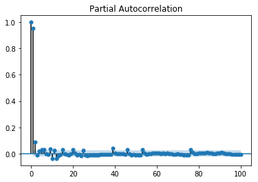
A partial auto-correlation is read in the same way as a correlogram.