- Time Series - Home
- Time Series - Introduction
- Time Series - Programming Languages
- Time Series - Python Libraries
- Data Processing & Visualization
- Time Series - Modeling
- Time Series - Parameter Calibration
- Time Series - Naive Methods
- Time Series - Auto Regression
- Time Series - Moving Average
- Time Series - ARIMA
- Time Series - Variations of ARIMA
- Time Series - Exponential Smoothing
- Time Series - Walk Forward Validation
- Time Series - Prophet Model
- Time Series - LSTM Model
- Time Series - Error Metrics
- Time Series - Applications
- Time Series - Further Scope
- Time Series Useful Resources
- Time Series - Quick Guide
- Time Series - Useful Resources
- Time Series - Discussion
Time Series - ARIMA
We have already understood that for a stationary time series a variable at time t is a linear function of prior observations or residual errors. Hence it is time for us to combine the two and have an Auto-regressive moving average (ARMA) model.
However, at times the time series is not stationary, i.e the statistical properties of a series like mean, variance changes over time. And the statistical models we have studied so far assume the time series to be stationary, therefore, we can include a pre-processing step of differencing the time series to make it stationary. Now, it is important for us to find out whether the time series we are dealing with is stationary or not.
Various methods to find the stationarity of a time series are looking for seasonality or trend in the plot of time series, checking the difference in mean and variance for various time periods, Augmented Dickey-Fuller (ADF) test, KPSS test, Hursts exponent etc.
Let us see whether the temperature variable of our dataset is a stationary time series or not using ADF test.
In [74]:
from statsmodels.tsa.stattools import adfuller

result = adfuller(train)
print('ADF Statistic: %f' % result[0])
print('p-value: %f' % result[1])
print('Critical Values:')
for key, value In result[4].items()
   print('\t%s: %.3f' % (key, value))
ADF Statistic: -10.406056
p-value: 0.000000
Critical Values:
1%: -3.431
5%: -2.862
10%: -2.567
Now that we have run the ADF test, let us interpret the result. First we will compare the ADF Statistic with the critical values, a lower critical value tells us the series is most likely non-stationary. Next, we see the p-value. A p-value greater than 0.05 also suggests that the time series is non-stationary.
Alternatively, p-value less than or equal to 0.05, or ADF Statistic less than critical values suggest the time series is stationary.
Hence, the time series we are dealing with is already stationary. In case of stationary time series, we set the d parameter as 0.
We can also confirm the stationarity of time series using Hurst exponent.
In [75]:
import hurst

H, c,data = hurst.compute_Hc(train)
print("H = {:.4f}, c = {:.4f}".format(H,c))
H = 0.1660, c = 5.0740
The value of H<0.5 shows anti-persistent behavior, and H>0.5 shows persistent behavior or a trending series. H=0.5 shows random walk/Brownian motion. The value of H<0.5, confirming that our series is stationary.
For non-stationary time series, we set d parameter as 1. Also, the value of the auto-regressive trend parameter p and the moving average trend parameter q, is calculated on the stationary time series i.e by plotting ACP and PACP after differencing the time series.
ARIMA Model, which is characterized by 3 parameter, (p,d,q) are now clear to us, so let us model our time series and predict the future values of temperature.
In [156]:
from statsmodels.tsa.arima_model import ARIMA

model = ARIMA(train.values, order=(5, 0, 2))
model_fit = model.fit(disp=False)
In [157]:
predictions = model_fit.predict(len(test))
test_ = pandas.DataFrame(test)
test_['predictions'] = predictions[0:1871]
In [158]:
plt.plot(df['T'])
plt.plot(test_.predictions)
plt.show()
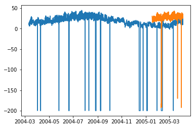
In [167]:
error = sqrt(metrics.mean_squared_error(test.values,predictions[0:1871]))
print ('Test RMSE for ARIMA: ', error)
Test RMSE for ARIMA: 43.21252940234892
