- TensorFlow - Home
- TensorFlow - Introduction
- TensorFlow - Installation
- Understanding Artificial Intelligence
- Mathematical Foundations
- Machine Learning & Deep Learning
- TensorFlow - Basics
- Convolutional Neural Networks
- Recurrent Neural Networks
- TensorBoard Visualization
- TensorFlow - Word Embedding
- Single Layer Perceptron
- TensorFlow - Linear Regression
- TFLearn and its installation
- CNN and RNN Difference
- TensorFlow - Keras
- TensorFlow - Distributed Computing
- TensorFlow - Exporting
- Multi-Layer Perceptron Learning
- Hidden Layers of Perceptron
- TensorFlow - Optimizers
- TensorFlow - XOR Implementation
- Gradient Descent Optimization
- TensorFlow - Forming Graphs
- Image Recognition using TensorFlow
- Recommendations for Neural Network Training
TensorFlow - TFLearn And Its Installation
TFLearn can be defined as a modular and transparent deep learning aspect used in TensorFlow framework. The main motive of TFLearn is to provide a higher level API to TensorFlow for facilitating and showing up new experiments.
Consider the following important features of TFLearn −
TFLearn is easy to use and understand.
It includes easy concepts to build highly modular network layers, optimizers and various metrics embedded within them.
It includes full transparency with TensorFlow work system.
It includes powerful helper functions to train the built in tensors which accept multiple inputs, outputs and optimizers.
It includes easy and beautiful graph visualization.
The graph visualization includes various details of weights, gradients and activations.
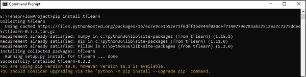
Install TFLearn by executing the following command −
pip install tflearn
Upon execution of the above code, the following output will be generated −
The following illustration shows the implementation of TFLearn with Random Forest classifier −
from __future__ import division, print_function, absolute_import

#TFLearn module implementation
import tflearn
from tflearn.estimators import RandomForestClassifier

# Data loading and pre-processing with respect to dataset
import tflearn.datasets.mnist as mnist
X, Y, testX, testY = mnist.load_data(one_hot = False)

m = RandomForestClassifier(n_estimators = 100, max_nodes = 1000)
m.fit(X, Y, batch_size = 10000, display_step = 10)

print("Compute the accuracy on train data:")
print(m.evaluate(X, Y, tflearn.accuracy_op))

print("Compute the accuracy on test set:")
print(m.evaluate(testX, testY, tflearn.accuracy_op))

print("Digits for test images id 0 to 5:")
print(m.predict(testX[:5]))

print("True digits:")
print(testY[:5])
