- NumPy - Home
- NumPy - Introduction
- NumPy - Environment
- NumPy Arrays
- NumPy - Ndarray Object
- NumPy - Data Types
- NumPy Creating and Manipulating Arrays
- NumPy - Array Creation Routines
- NumPy - Array Manipulation
- NumPy - Array from Existing Data
- NumPy - Array From Numerical Ranges
- NumPy - Iterating Over Array
- NumPy - Reshaping Arrays
- NumPy - Concatenating Arrays
- NumPy - Stacking Arrays
- NumPy - Splitting Arrays
- NumPy - Flattening Arrays
- NumPy - Transposing Arrays
- NumPy Indexing & Slicing
- NumPy - Indexing & Slicing
- NumPy - Indexing
- NumPy - Slicing
- NumPy - Advanced Indexing
- NumPy - Fancy Indexing
- NumPy - Field Access
- NumPy - Slicing with Boolean Arrays
- NumPy Array Attributes & Operations
- NumPy - Array Attributes
- NumPy - Array Shape
- NumPy - Array Size
- NumPy - Array Strides
- NumPy - Array Itemsize
- NumPy - Broadcasting
- NumPy - Arithmetic Operations
- NumPy - Array Addition
- NumPy - Array Subtraction
- NumPy - Array Multiplication
- NumPy - Array Division
- NumPy Advanced Array Operations
- NumPy - Swapping Axes of Arrays
- NumPy - Byte Swapping
- NumPy - Copies & Views
- NumPy - Element-wise Array Comparisons
- NumPy - Filtering Arrays
- NumPy - Joining Arrays
- NumPy - Sort, Search & Counting Functions
- NumPy - Searching Arrays
- NumPy - Union of Arrays
- NumPy - Finding Unique Rows
- NumPy - Creating Datetime Arrays
- NumPy - Binary Operators
- NumPy - String Functions
- NumPy - Matrix Library
- NumPy - Linear Algebra
- NumPy - Matplotlib
- NumPy - Histogram Using Matplotlib
- NumPy Sorting and Advanced Manipulation
- NumPy - Sorting Arrays
- NumPy - Sorting along an axis
- NumPy - Sorting with Fancy Indexing
- NumPy - Structured Arrays
- NumPy - Creating Structured Arrays
- NumPy - Manipulating Structured Arrays
- NumPy - Record Arrays
- Numpy - Loading Arrays
- Numpy - Saving Arrays
- NumPy - Append Values to an Array
- NumPy - Swap Columns of Array
- NumPy - Insert Axes to an Array
- NumPy Handling Missing Data
- NumPy - Handling Missing Data
- NumPy - Identifying Missing Values
- NumPy - Removing Missing Data
- NumPy - Imputing Missing Data
- NumPy Performance Optimization
- NumPy - Performance Optimization with Arrays
- NumPy - Vectorization with Arrays
- NumPy - Memory Layout of Arrays
- Numpy Linear Algebra
- NumPy - Linear Algebra
- NumPy - Matrix Library
- NumPy - Matrix Addition
- NumPy - Matrix Subtraction
- NumPy - Matrix Multiplication
- NumPy - Element-wise Matrix Operations
- NumPy - Dot Product
- NumPy - Matrix Inversion
- NumPy - Determinant Calculation
- NumPy - Eigenvalues
- NumPy - Eigenvectors
- NumPy - Singular Value Decomposition
- NumPy - Solving Linear Equations
- NumPy - Matrix Norms
- NumPy Element-wise Matrix Operations
- NumPy - Sum
- NumPy - Mean
- NumPy - Median
- NumPy - Min
- NumPy - Max
- NumPy Set Operations
- NumPy - Unique Elements
- NumPy - Intersection
- NumPy - Union
- NumPy - Difference
- NumPy Random Number Generation
- NumPy - Random Generator
- NumPy - Permutations & Shuffling
- NumPy - Uniform distribution
- NumPy - Normal distribution
- NumPy - Binomial distribution
- NumPy - Poisson distribution
- NumPy - Exponential distribution
- NumPy - Rayleigh Distribution
- NumPy - Logistic Distribution
- NumPy - Pareto Distribution
- NumPy - Visualize Distributions With Sea born
- NumPy - Matplotlib
- NumPy - Multinomial Distribution
- NumPy - Chi Square Distribution
- NumPy - Zipf Distribution
- NumPy File Input & Output
- NumPy - I/O with NumPy
- NumPy - Reading Data from Files
- NumPy - Writing Data to Files
- NumPy - File Formats Supported
- NumPy Mathematical Functions
- NumPy - Mathematical Functions
- NumPy - Trigonometric functions
- NumPy - Exponential Functions
- NumPy - Logarithmic Functions
- NumPy - Hyperbolic functions
- NumPy - Rounding functions
- NumPy Fourier Transforms
- NumPy - Discrete Fourier Transform (DFT)
- NumPy - Fast Fourier Transform (FFT)
- NumPy - Inverse Fourier Transform
- NumPy - Fourier Series and Transforms
- NumPy - Signal Processing Applications
- NumPy - Convolution
- NumPy Polynomials
- NumPy - Polynomial Representation
- NumPy - Polynomial Operations
- NumPy - Finding Roots of Polynomials
- NumPy - Evaluating Polynomials
- NumPy Statistics
- NumPy - Statistical Functions
- NumPy - Descriptive Statistics
- NumPy Datetime
- NumPy - Basics of Date and Time
- NumPy - Representing Date & Time
- NumPy - Date & Time Arithmetic
- NumPy - Indexing with Datetime
- NumPy - Time Zone Handling
- NumPy - Time Series Analysis
- NumPy - Working with Time Deltas
- NumPy - Handling Leap Seconds
- NumPy - Vectorized Operations with Datetimes
- NumPy ufunc
- NumPy - ufunc Introduction
- NumPy - Creating Universal Functions (ufunc)
- NumPy - Arithmetic Universal Function (ufunc)
- NumPy - Rounding Decimal ufunc
- NumPy - Logarithmic Universal Function (ufunc)
- NumPy - Summation Universal Function (ufunc)
- NumPy - Product Universal Function (ufunc)
- NumPy - Difference Universal Function (ufunc)
- NumPy - Finding LCM with ufunc
- NumPy - ufunc Finding GCD
- NumPy - ufunc Trigonometric
- NumPy - Hyperbolic ufunc
- NumPy - Set Operations ufunc
- NumPy Useful Resources
- NumPy - Quick Guide
- NumPy - Cheatsheet
- NumPy - Useful Resources
- NumPy - Discussion
- NumPy Compiler
NumPy - Pareto Distribution
What is Pareto Distribution?
The Pareto Distribution is a continuous probability distribution used to model the distribution of wealth, income, or other resources, where a small portion of the population controls a large proportion of the total.
It is defined by two parameters: the shape parameter and the scale parameter xm. The distribution is known for its "80/20 rule," where roughly 80% of the effects come from 20% of the causes.
Example: The Pareto distribution can model the distribution of wealth in a population, where a few individuals hold most of the wealth.
The probability density function (PDF) of the Pareto distribution is −
f(x; , xm) = ( * xm) / x+1, for x xm
Where,
- : Shape parameter, which determines the steepness of the distribution's tail.
- xm: Scale parameter, which represents the minimum value of the distribution (also known as the "threshold").
- x: Random variable representing the value we are interested in.
- + 1: The exponent of the random variable, showing the heavy-tailed nature of the distribution.
The Pareto distribution is commonly used in the modeling of "rich-get-richer" phenomena, where the probability of a value decreases rapidly as the value increases.
Pareto Distributions in NumPy
NumPy provides a built-in function numpy.random.pareto() function to generate random samples from the Pareto distribution. You need to specify the shape parameter and scale parameter xm. The function will generate random values according to the Pareto distribution.
Example
In this example, we generate 10 random samples from the Pareto distribution with a shape parameter () of 2 and a scale parameter (xm) of 1. Since the Pareto distribution is defined for values greater than or equal to xm, we add 1 to shift the distribution to start at 1 −
import numpy as np

# Generate 10 random samples from a Pareto distribution with shape parameter =2 and scale parameter xm=1
samples = np.random.pareto(a=2, size=10) + 1  # xm=1, we add 1 to shift the distribution
print("Random samples from Pareto distribution:", samples)
Following is the output obtained −
Random samples from Pareto distribution: [11.21752644  1.19133192  1.13107575  1.00672706  1.77411845  1.29541783
  5.99272696  1.62119397  1.08409404  1.25025651]
Visualizing Pareto Distributions
Visualization is an important tool to understand the characteristics of distributions. We can visualize the Pareto distribution by creating histograms using Matplotlib.
Example
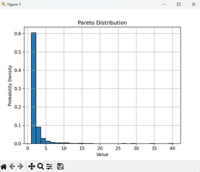
In the following example, we are first generating 1000 random samples from a Pareto distribution. We are then creating a histogram of the samples to visualize this distribution −
import numpy as np
import matplotlib.pyplot as plt

# Generate 1000 random samples from a Pareto distribution
samples = np.random.pareto(a=2, size=1000) + 1

# Plot the histogram of the samples
plt.hist(samples, bins=30, density=True, edgecolor='black')
plt.title('Pareto Distribution')
plt.xlabel('Value')
plt.ylabel('Probability Density')
plt.grid(True)
plt.show()
The histogram shows the probability density of the generated values. As expected, the distribution has a "heavy tail," meaning that a small number of larger values contribute significantly to the total probability. The distribution decays quickly as the values increase −
Parameters of the Pareto Distribution
The two parameters of the Pareto distribution, and xm, plays an important role in shaping the distribution. Let us break down how each parameter affects the distribution −
- Shape Parameter (): The shape parameter controls the steepness of the distribution's tail. As increases, the tail becomes steeper, and the distribution becomes less "heavy-tailed." A smaller results in a distribution with a heavier tail and more extreme values.
- Scale Parameter (xm): The scale parameter sets the minimum value for the distribution. A higher xm shifts the distribution to the right, meaning that the random samples will only take values greater than or equal to this threshold.
Applications of Pareto Distribution
The Pareto distribution has many practical applications in modeling and data analysis −
- Economics: The Pareto distribution is often used to model income distribution, wealth distribution, and other economic phenomena where a small portion of the population controls a large proportion of the wealth.
- Network Traffic: It can be used to model internet traffic, where a small number of users generate the majority of the data.
- Insurance: The Pareto distribution is applied in risk modeling, particularly in areas like natural disasters, where large losses are rare but significant.
- Engineering: It is used to model component failures in engineering, where a few components fail frequently while the rest have long lifespans.
Statistical Properties of the Pareto Distribution
Like other distributions, the Pareto distribution has some interesting statistical properties −
- Mean: The mean of the Pareto distribution is * xm / ( - 1) for > 1. If 1, the mean is undefined because the distribution has a heavy tail.
- Variance: The variance of the Pareto distribution is * xm / (( - 1) * ( - 2)) for > 2. If 2, the variance is infinite due to the heavy tail.
- Skewness: The Pareto distribution is skewed to the right, meaning it has a long tail on the positive side.
Generating a Pareto Distribution with Custom Parameters
You can modify the shape and scale parameters to generate Pareto distributions that better reflect your data.
Example
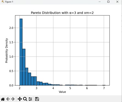
Following is an example where we set =3 and xm=2 to generate a pareto distribution −
import numpy as np
import matplotlib.pyplot as plt

# Generate 1000 random samples with =3 and xm=2
samples = np.random.pareto(a=3, size=1000) + 2

# Plot the histogram of the samples
plt.hist(samples, bins=30, density=True, edgecolor='black')
plt.title('Pareto Distribution with =3 and xm=2')
plt.xlabel('Value')
plt.ylabel('Probability Density')
plt.grid(True)
plt.show()
This graph will show a distribution with a slightly less heavy tail than the one with =2 and xm=1 −
Seeding for Reproducibility
For reproducibility, it is important to set a random seed. This ensures that every time you run the code, you get the same set of random numbers.
Example
By setting the seed, you ensure that the random generation produces the same result every time the code is executed as shown in the example below −
import numpy as np

# Set the seed for reproducibility
np.random.seed(42)

# Generate 10 random samples with =2 and xm=1
samples = np.random.pareto(a=2, size=10) + 1
print("Random samples from Pareto distribution with seed:", samples)
The result produced is as follows −
Random samples from Pareto distribution with seed: [1.26444595 4.50442711 1.93164669 1.57849408 1.08851288 1.08849733
 1.03037147 2.73358909 1.58334718 1.85081305]
