
Article Categories
- All Categories
-
 Data Structure
-
 Networking
-
 RDBMS
RDBMS
-
 Operating System
-
 Java
Java
-
 MS Excel
-
 iOS
iOS
-
 HTML
HTML
-
 CSS
CSS
-
 Android
-
 Python
-
 C Programming
-
 C++
C++
-
 C#
C#
-
 MongoDB
-
 MySQL
MySQL
-
 Javascript
-
 PHP
PHP
-
 Economics & Finance
How to look up partial string match in excel?
In Excel, sometimes the user needs to search for a specific value that only partially matches the data in a range. This can be done using the powerful combination of the INDEX and MATCH functions. By leveraging these functions, the user can easily perform partial string matching to retrieve desired information from our Excel spreadsheets. Here, will be using a simple example to demonstrate the process of looking at partial string matching in Excel.
Example 1: To look up the partial string match in Excel by using the user-defined formula.
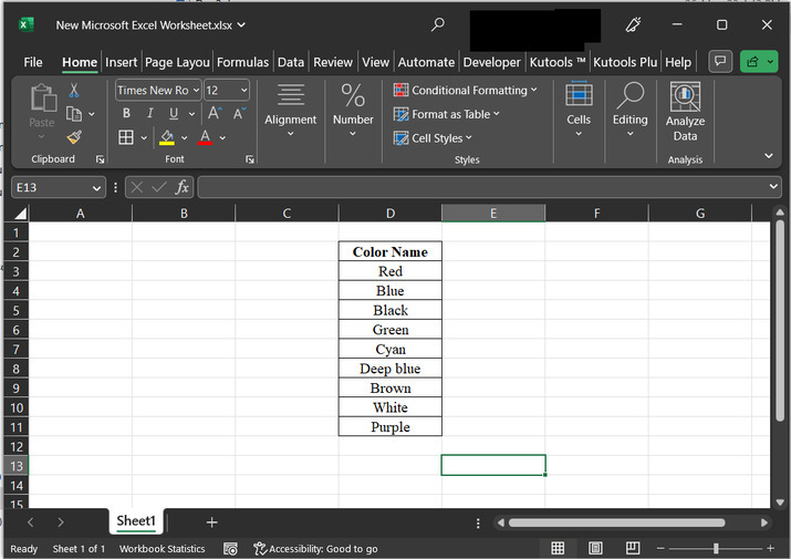
Step 1
In this example, the user will learn the process of looking up partial-string matches in Excel, by using the user defined formula. To do so, consider the given excel sheet below. This Excel sheet contains a column that stores color names. In this example, the user will try to pass a partial string to obtain a required color name.
Step 2
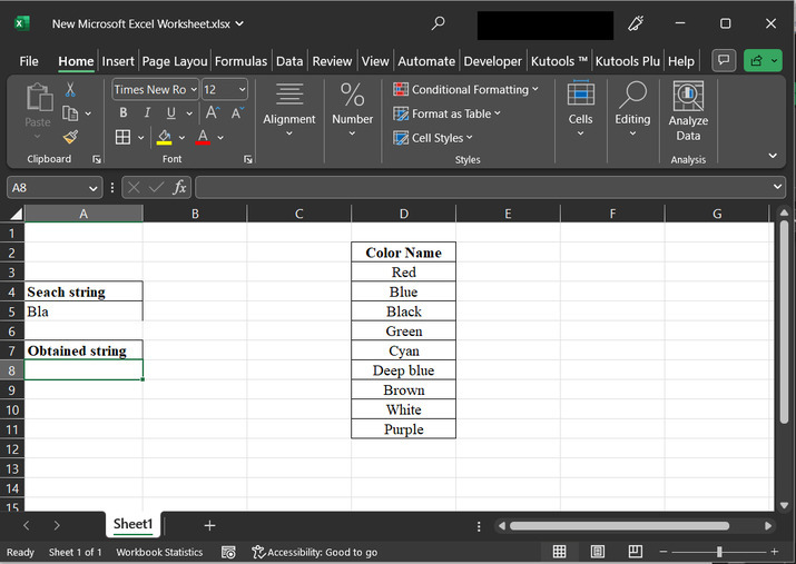
In the next step will create two separate column headers. Go to cell A4, and type the column header for "search string". After that in the A5 cell write "Bla". In this example, will pass the partial string "Bla", and from column D extract a complete equivalent string. Then go to cell A7, and type "Obtained String". Obtained results will be printed on the A8 cell. consider below provided snapshot for proper reference ?
Step 3
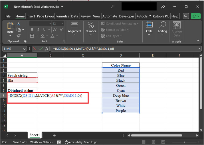
Go to the A8 cell, and type formula "=INDEX(D3:D11,MATCH(A5&"*",D3:D11,0))". As shown below ?
Explanation for above formula:
The used formula "=INDEX(D3:D11, MATCH(A5&"*", D3:D11, 0))" is an Excel formula.
Let's break down the formula:
"=INDEX (D3:D11," - This part indicates that user wants to use the INDEX function to return a value from the range D3:D11.
"MATCH (A5 & "", D3:D11, 0)" - This part is the MATCH function, which searches for a specified value (in this case, A5 concatenated with an asterisk "") within the range D3:D11. The "&" operator is used for concatenation, so it combines the value in cell A5 with the asterisk. The asterisk is a wildcard character that matches any number of characters. The "0" at the end indicates that we want an exact match.
Putting it all together, the formula searches for the value in cell A5 followed by any additional characters (using the asterisk wildcard) within the range D3:D11. If it finds a match, the INDEX function returns the corresponding value from the range D3:D11.
Step 3
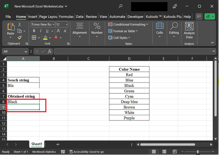
After typing the formula, press the "Enter" key. This will display the data value "black" to the A8 cell. As Black is equivalent to the partial passes string "bla".
Conclusion
In conclusion, the formula "=INDEX(D3:D11, MATCH(A5&"*", D3:D11, 0))" provides a practical solution for performing partial string matching in Excel. By using the INDEX and MATCH functions together, the user can search for a specific value that partially matches the data in a range and retrieve the corresponding information from another range. This technique enhances our ability to work with data efficiently, enabling us to find and analyze information more effectively in Excel spreadsheets.

10K+ Views
