How to Quickly Sort Rows to Match Another Column in Excel?

In this article, the user will learn the process of sorting rows by matching the data with another column. Sorting rows to match the content of another column in Excel can be a powerful technique whenever a user needs to organize and align data efficiently. Whether the user has a dataset with related information in separate columns or in a case needs to arrange data according to a specific reference column. With the help of Excel, users can perform this task efficiently. By leveraging sorting functions, users can quickly restructure the data to make the data useful for analysis, comparison, and visualization. This article provides a simple illustration to explain the required task briefly in a stepwise manner.

Example 1: To quickly sort the rows to match another in excel by using the user defined formula, and sort feature:

Step 1

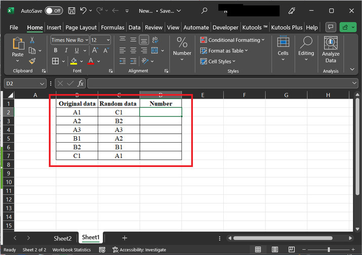
This article allows user to sort the rows to match to another column in excel. In this example, will assume that the data available in the first column stores the data with column header as original data, second column contains data for random data, and the third column stores data for number values. Snapshot for the data is provided below:

Step 2

Go to the D2 cell, and type “=MATCH(C2,$B$2:$B$7,0)”. Snapshot for user reference is provided below:

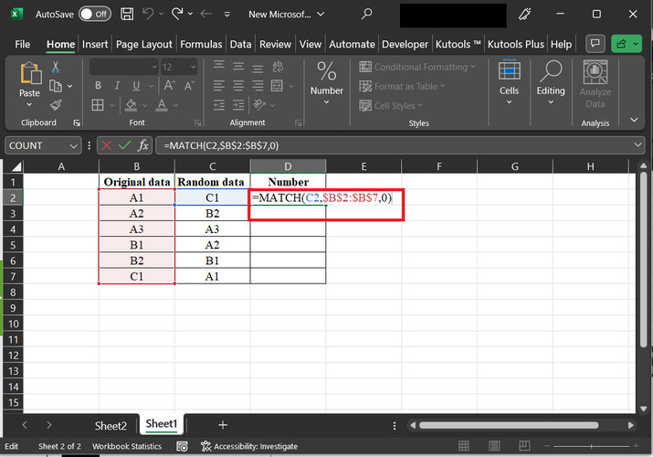
Explanation for formula “=MATCH(C2,$B$2:$B$7,0)”

The formula "=MATCH(C2, $B$2:$B$7, 0)" is used in Excel to determine the position of a value in a specified range.

• "C2": This is a cell reference to cell C2, that contains the value that user want to determine in the range.

• "$B$2:$B$7": This is the range by using which user can search for the value. In this case, the range is from cell B2 to B7.

• "0": The last argument of the MATCH function is the match type. In this case, "0" (zero) indicates that an exact match is required. It means that the function will look for the value in C2 and determine the first occurrence of that exact value in the range B2:B7.

Step 3

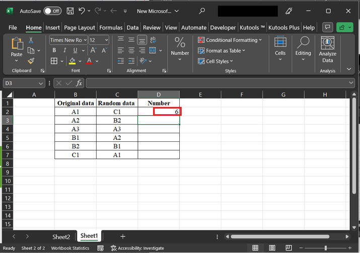
The above provided formula will generate result value as 6. Snapshot for reference is provided below:

Step 4

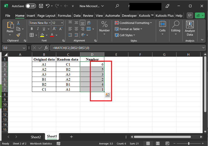
Drag the fill handle to display the results accordingly. Snapshot for reference is provided below:

Step 5

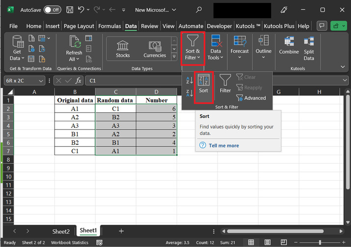
After that go to the “Data” tab, and then click on the “Sort” option. A snapshot for same is provided below:

Step 6

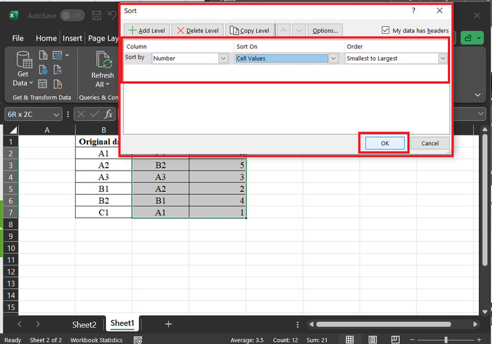
The above step will open a sort dialog box. After that go to the column label, go to the sort by label, choose “Number”, go to the label sort on, and choose option “Cell Values”. After that click on the order label, and click on the option “Smallest to Largest”. After that click on the “OK” button. A snapshot for reference is provided below:

Step 7

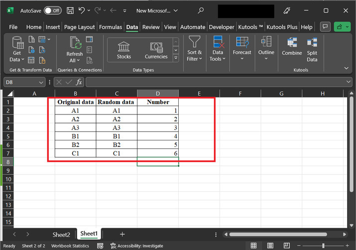
The final sorted snapshot of data is provided below:

Conclusion

This article illustrates the process of sorting the rows to match another column’s data. All the provided steps are accurate, detailed, and thorough. Tasks can be done easily by referring to all the provided steps manually. All the processing steps are shown with the help of snapshots precisely.