How to use the Filter Function for a complete match and Partial Match of Text string in Excel?

The filter function is a newly introduced function in Excel 2021 and Excel 365. In this article, we will understand the fundamental concept of the Filter function which is efficient in finding the filtered string presented in the dataset that relies on the specific criteria and extracts only those searched strings. This interesting function is compatible with other functions like Search, Match, ISNUMBER, and so on. The process of manually scanning a text string from a huge dataset is time-consuming and inefficient for the user. In addition to saving users time, the filter tool allows users to find an accurate match more quickly.

Filter function for complete match of String

Step 1

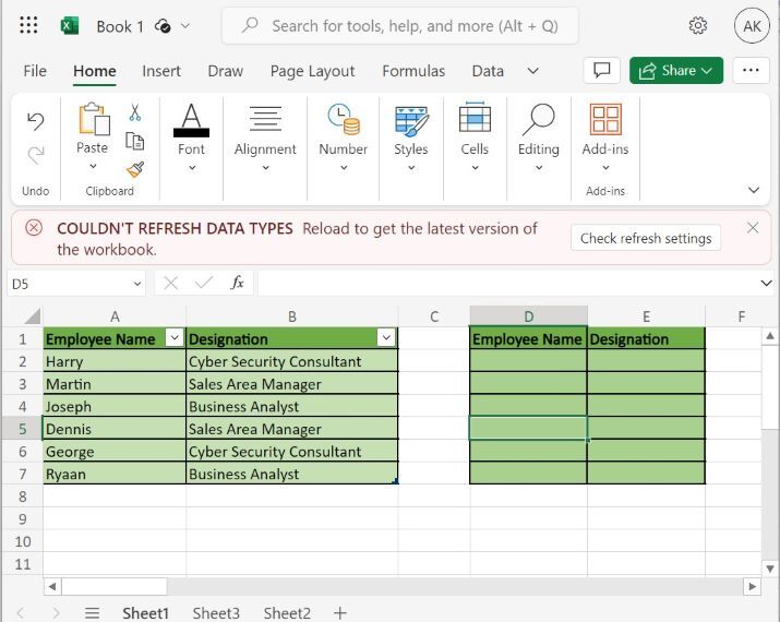
Users need to open a new worksheet in Excel 365 and create a table comprising two columns “Employees Name” and “Designation”. Enter the corresponding entries in these two columns range A2:B7. Similarly, develop another table in the range D1:E7 as shown below −

Step 2

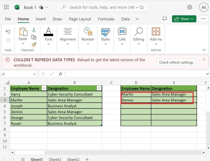
The user would write the formula =FILTER(Table2,Table2[Designation]="Sales Area Manager") in the D2 cell and then press the “Enter” tab to obtain the list of those employees whose designation is “Sales Area Manager”.

Explanation

=FILTER(Table2,Table2[Designation]="Sales Area Manager") 

• Table2 − The first argument specifies the complete range A2:B7 of the table.

• Table2[Designation]="Sales Area Manager") − The second argument denotes Table 2’s second column named “Designation” and searches only those designation which is equal to the “Sales Area Manager”.

Partial match by using the Filter function

Step 1

Assume the same table as defined in the previous example.

Step 2

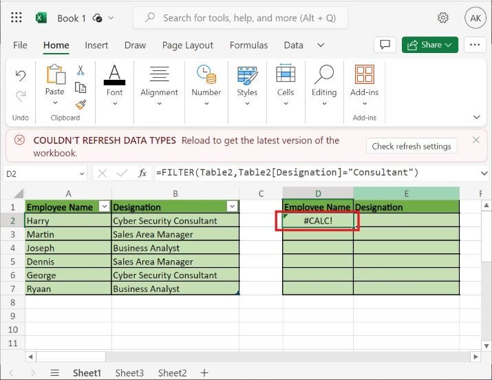
Suppose we write the formula “=FILTER(Table2,Table2[Designation]="Consultant")” for the partial match in the D2 cell. Press the “Enter” tab but an error may arise in the result.

Step 3

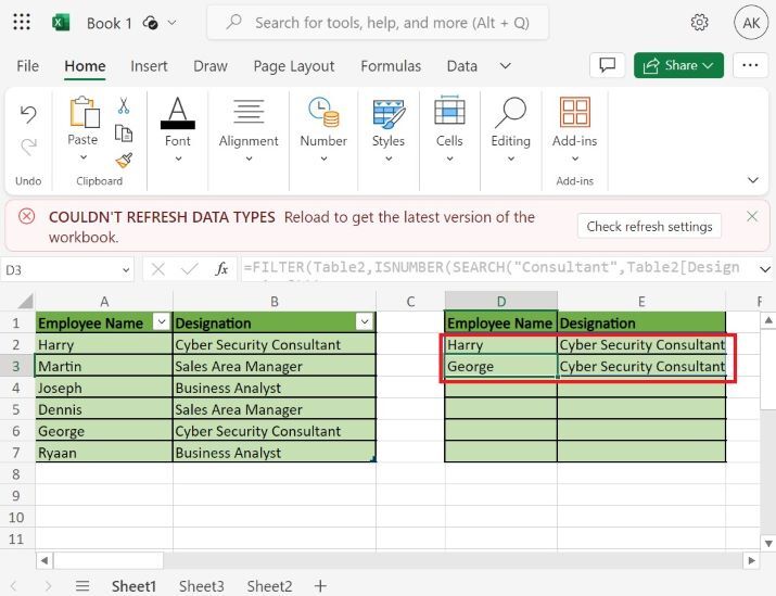
To eliminate this error, write the formula =FILTER(Table2,ISNUMBER(SEARCH("Consultant",Table2[Designation]))) in the D2 cell as highlighted in below image −

Explanation

=FILTER(Table2,ISNUMBER(SEARCH("Consultant",Table2[Designation])))

• The first argument is Table2 indicating the range “A2:B7”.

• The second argument defines another “ISNUMBER” function that returns true if the nested search function’s condition is correct. Otherwise, it would return False.

• The Search function finds only those texts whose value is “Consultant” in the second column of the Table.

• After utilizing the complete formula, only those employee names along with designations are extracted whose designation contains the partial text “Consultant”.

Step 4

When we press the “Enter” tab, we obtain the accurate result as given below −

Conclusion

The two examples are demonstrated in this article. Users would master Excel proficiency through these tricky techniques. The filter function works independently if the user must find the entire text string. However, for partial matches, users can employ the ISNUMBER and Search functions inside the Filter function as depicted in the second example.