How to match dates by month and year only in Excel?

Sometimes we need to find the similar dates in dataset of multiple dates to identify the frequency of occurrence of any activity in a month/year or day. For this we have a formula in excel using which we can instantly find out the dates falling under a specific year and/or month even for a single day. We will be using the following two methods to identify the dates by month and year only from a dataset.

• Comparing adjacent dates by month and year only through a formula

• Finding dates by month and year only through Conditional Formatting

Finding Dates by Month and Year only through a Formula

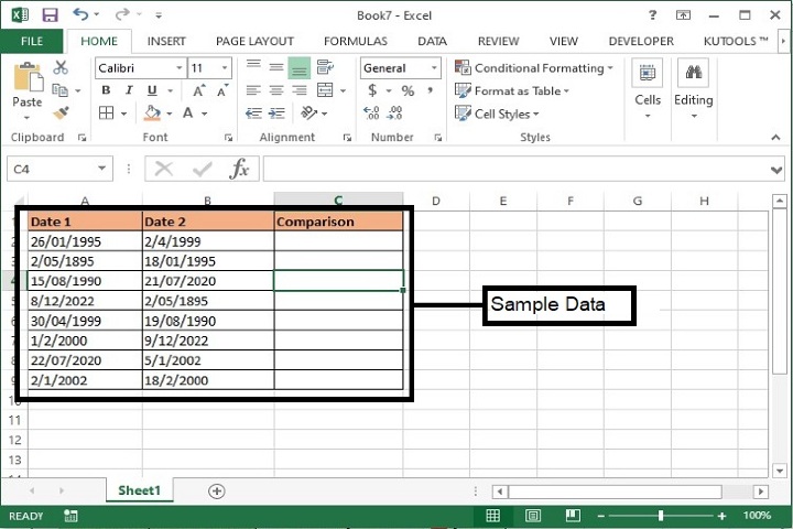
Step 1 − We have taken the following sample data having 3 columns as following −

• Date 1 − Group1 of some random dates

• Date 2 − Group2 of some random dates

• Comparison − Formula will be mentioned here to identify whether the adjacent dates match with month and year or not.

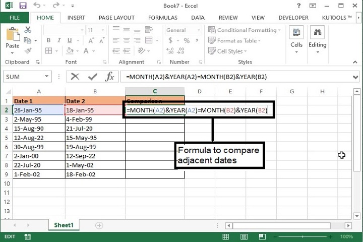
Step 2 − Under the column C enter the following formula at C2 cell and press enter.

=MONTH(A2)&YEAR(A2)=MONTH(B2)&YEAR(B2)

This formula will compare the month and year of adjacent cells of Date 1 and Date 2 columns.

Step 3 − Drag the formula till the last row. Now following will be the output.

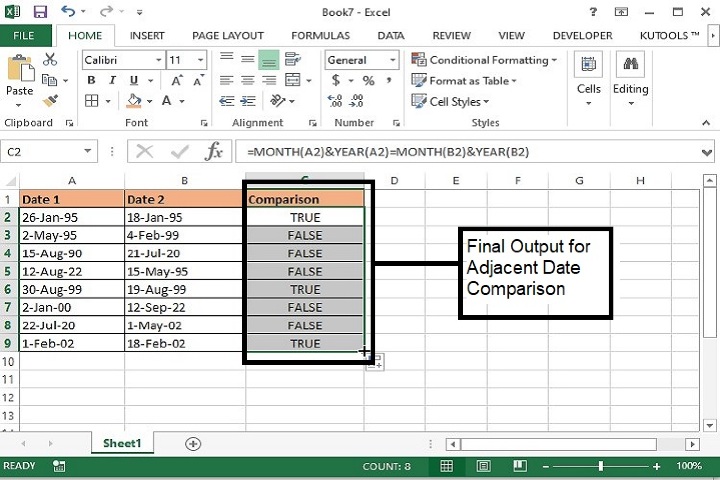
Here, True is returned when month and year of the adjacent dates match otherwise the system returns False.

Formula Syntax Description

Argument	Description
MONTH(serial_number)	Against serial number, mention a cell address with date value and it will return the month of the respective date.
YEAR(serial_number)	Against serial number, mention a cell address with date value and it will return the year of the respective date.

Finding Dates by Month and Year only through Conditional Formatting

Using this formula we can search and highlight all the dates having similar month and year as compared to a specific date. Let’s see how this can be achieved.

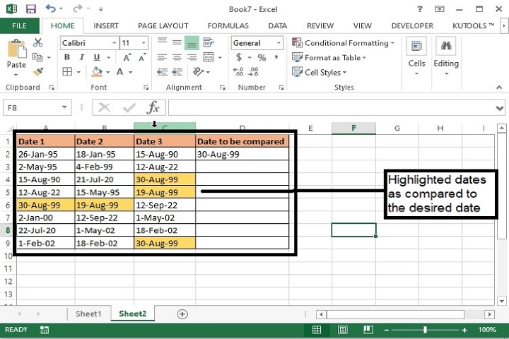
Step 1 − Following is the sample data where we have four columns as following −

• Date 1 − Date set 1

• Date 2 − Date set 2

• Date 3 − Date set 3

• Date to be compared − Specific date which will be compared.

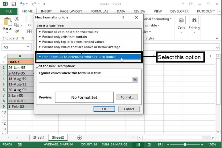
Step 2 − Now select the date sets with which specific date needs to be compared and go to Home / Conditional Formatting / New Rule.

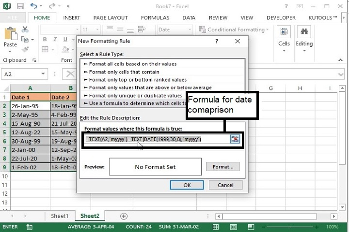
Step 3 − In the New Formatting Rule dialog box, select Use a formula to determine which cells to format under select a rule type.

Step 4 − Enter the following formula under the field, Format values where this formula is true.

=TEXT(A2,"myyyy")=TEXT(DATE(1999,30,8),"myyyy")

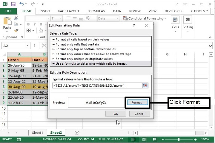
Step 5 − After entering the formula click Format against Preview field.

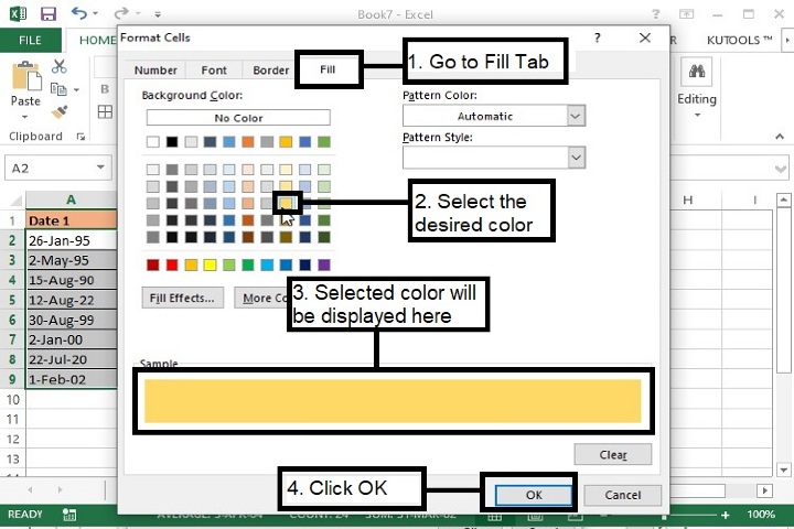
Step 6 − On click of Format, following dialog box will open. Here go to the ‘Fill’ tab select the color to highlight the matched dates as shown below and click OK.

The preview of New rule will be as following. Here, click OK.

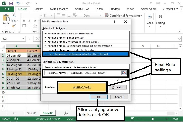
Step 7 − The final output will be as following where all the dates having month and year similar to the selected date have been highlighted.

Conclusion

Please note that in the formula, A2 is the first cell of selected date range, 1999,8,30 is the given date we have compared with. Please change them based on your requirement. This method is more useful than the previous one as it compares the date with a set of dates instead of just one value. However, it depends completely on your requirement which ever suits you