
Article Categories
- All Categories
-
 Data Structure
-
 Networking
-
 RDBMS
RDBMS
-
 Operating System
-
 Java
Java
-
 MS Excel
-
 iOS
iOS
-
 HTML
HTML
-
 CSS
CSS
-
 Android
-
 Python
-
 C Programming
-
 C++
C++
-
 C#
C#
-
 MongoDB
-
 MySQL
MySQL
-
 Javascript
-
 PHP
PHP
-
 Economics & Finance
How to Look up the First Non-Zero Value and Return Corresponding Column Header in Excel?
In this article, users would easily look up the first non-zero value in a row and obtain the corresponding column header. One example is showcased in this article that facilitates efficient solutions for working with data in Excel. By using the combination of the INDEX and MATCH functions in Excel, the provided formula allows the user to determine the column header associated with the first non-zero value in a specific row. By adjusting the ranges to match the data, the user can apply this formula across multiple rows or ranges, helping the user to analyze and process data based on specific criteria.
Example 1: To look up the first non-zero value column header in Excel by using the user-defined formula.
Step 1
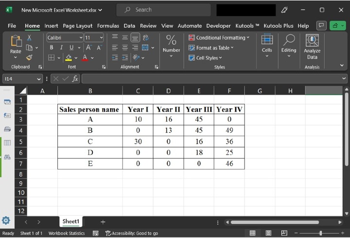
To understand the process of calculating the first non-zero value column header in Excel, consider the below provided Excel spreadsheet. In the available Excel sheet, there are a total of 5 columns. Here, the first column contains the name of a salesperson. While the rest 4 columns contain the sales number for each salesperson in a different month.
Step 2
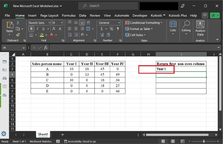
To store the calculated result, let?s create a separate column header. To do so, go to the I2 cell, and write "Return first non-zero column", as provided below:

Step 3
Now, go to the I3, cell and type "=INDEX(C2:F2,MATCH(TRUE,INDEX(C3:F3<>0,),0))" formula in the Excel sheet. To understand more precisely consider the below-provided snapshot:

The explanation for the provided formula:
C3:F3<>0 checks each cell in the range C3:F3 to determine if it is not equal to zero. This creates an array of TRUE/FALSE values, with TRUE, indicating a non-zero value and FALSE indicating a zero value.
MATCH(TRUE, C3:F3<>0, 0) searches for the position of the first TRUE value in the array created by the previous step. It returns the relative position of the first non-zero value found in the range C3:F3.
INDEX(C2:F2, MATCH(TRUE, C3:F3<>0, 0)) uses the position returned by the MATCH function to retrieve the corresponding value from the range C2:F2. The INDEX function returns the value located at the intersection of the row C2:F2 and the column determined by the position of the first non-zero value in C3:F3.
Step 4
Press the "Enter" key to display the calculated results on the Excel sheet. Consider the below-given snapshot of the code:
Conclusion
This technique is particularly valuable when dealing with large datasets or performing calculations that depend on identifying key values. By leveraging the power of Excel's functions, the user can streamline their data analysis workflow and extract the information user need efficiently.
By mastering this method, users can enhance individual?s Excel skills and gain a better understanding of data, by enabling users to make informed decisions and perform various calculations or operations based on the first non-zero value and its corresponding column header.

8K+ Views
