How to look up a value and return the cell above or below in excel?

In this article, the user will take deep practical knowledge of how to look for a value and return the cell above or below in Excel. This article will briefly two examples. The first example demonstrates the process of generating the above cell value in Excel by using the user-defined formula, while the second example demonstrates the process of generating the below cell value in an Excel sheet. Consider the below provided detailed stepwise explanation, to understand the process briefly.

Example 1: To look up for a value in excel sheet, and returning the cell value above to the specified cell

Step 1

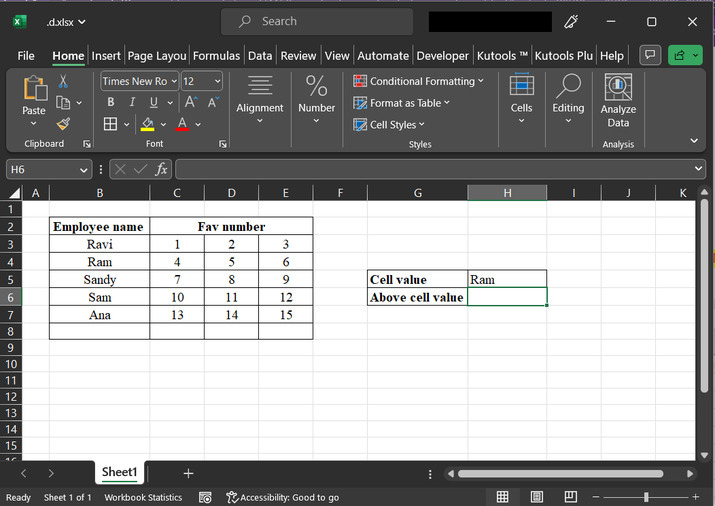
To state the stepwise explanation, consider the below given snapshot of the Excel sheet. The given Excel sheet will take two main columns. The first column contains the name of an employee, while the second column contains, three sub-columns that together store the favorite number of employees.

Step 2

This step, will guide the user to make a cell header for value, above which the data is to be looked inside the table, as specified above. After that go to the G6 cell header. This cell header will store the generated data value. Consider the below given snapshot −

Step 3

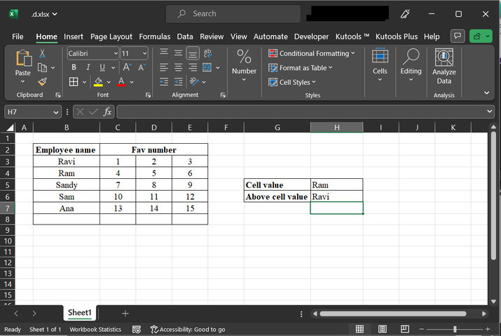
Go to the H6 cell, and type formula “=INDEX(B3:B7,MATCH(H5,B3:B7,0)-1,1)”. In the cell, a snapshot for the same is provided below −

The explanation for the required formula:

The above-provided formula in Excel is used to find a value in the range B3:B7 and return the value from the cell directly above it.

Let's break down the formula:

• INDEX(B3:B7, ...) specifies the range of cells B3:B7 from which we want to retrieve a value.

• MATCH(H5, B3:B7,0) searches for the value in cell H5 within the range B3:B7 and returns the position of the matched value.

• -1 is subtracted from the result of the MATCH function. This is done to adjust the position by moving one cell up to get the value from the cell above the matched value.

• 1 indicates that the user wants to obtain the value from the 1st column of the range B3:B7.

Step 4

And then simply press the “Enter” key.

Example 2: To look up a value in Excel sheet, and returning the cell value below the specified cell

Step 1

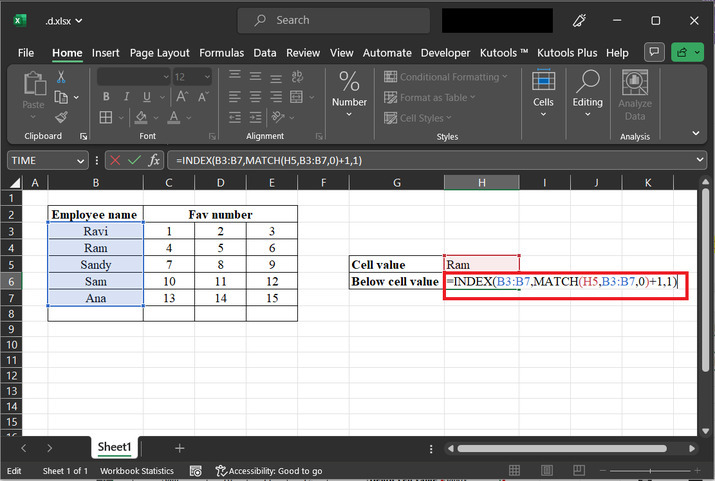
In this example, the user will understand the process using the formula, to calculate the value of the next cell. Assume the data as shown below −

Step 2

Go to the “H6” cell, and type the formula “=INDEX(B3:B7,MATCH(H5,B3:B7,0)+1,1)”. This formula will allow the user to calculate the next cell value −

Explanation for formula

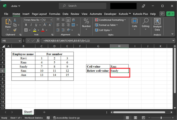
The above-described formula in Excel is used to search for a value in the range B3:B7. It returns the value from the cell directly below the matched value.

To break it down further

• MATCH(H5,B3:B7,0) searches for the value in cell H5 within the range B3:B7 and determines the position of the matched value.

• +1 is added to the result of the MATCH function to move one cell down from the matched position.

• INDEX(B3:B7, ...) retrieves the value from the range B3:B7 based on the adjusted position.

• ,1 specifies that the value to be returned is from the first column of the range.

In summary, the formula searches for a value in a specified range and returns the value from the cell immediately below the matched value.

Step 3

Press the “Enter” key to obtain the value next to the current cell value. Consider the snapshot provided below −

Conclusion

This article briefs two common examples, all the above-guided steps are accurate and precise. By following the steps precisely, the user can easily learn the process of looking up and down data values in any available dataset. Both examples are based on user-defined formulas Thus, the user needs to recognize and learn the formula properly before using it.