
 Data Structure
 Networking
 RDBMS
RDBMS Operating System
 Java
Java MS Excel
 iOS
iOS HTML
HTML CSS
CSS Android
 Python
 C Programming
 C++
C++ C#
C# MongoDB
 MySQL
MySQL Javascript
 PHP
PHP
- Selected Reading
- UPSC IAS Exams Notes
- Developer's Best Practices
- Questions and Answers
- Effective Resume Writing
- HR Interview Questions
- Computer Glossary
- Who is Who
How to insert image control in Excel?
In Excel, adding an image control generally refers to the process of adding an interactive image to a user form or a worksheet. The image control allows users to interact with the image, such as clicking, viewing, zooming, or performing other actions based on its presence.
In this article, the user will understand the process of inserting image control in the Excel sheet. This allows the user to insert any control to an image. For example, a macro can be assigned to the inserted image. So, whenever the user clicks on this image the macro will activate itself automatically, without any need to call the macro manually. This is the most important application of image control inserted in Excel. Sometimes image controls are used to improve the visual of the Excel sheet, and to make the sheet interactive.
This article contains a stepwise explanation for a task, by referring to all these steps, users can easily learn the way to insert an effective image control in Excel. Another major point to remember any self-created image can also be inserted into the Excel sheet. To do this, so user first needs to create an image, save it with the proper ".jpg" extension, and then save the file with the proper extension to a valid place, and remember the location, as the user needs to use the location, while importing the image to the excel sheet.
Example 1: To insert the image control in Excel by using the ActiveX controls available in the developer tab.
Step 1
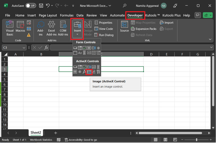
To insert the image control feature in Excel, consider an empty Excel sheet. In the empty Excel sheet, click on the "Developer" tab, and then select the "Insert" option. After that go to the "Active X Controls", and click on the image option, provided at the last third button in the Excel sheet. For proper reference consider the below provided excel sheet:
Step 2
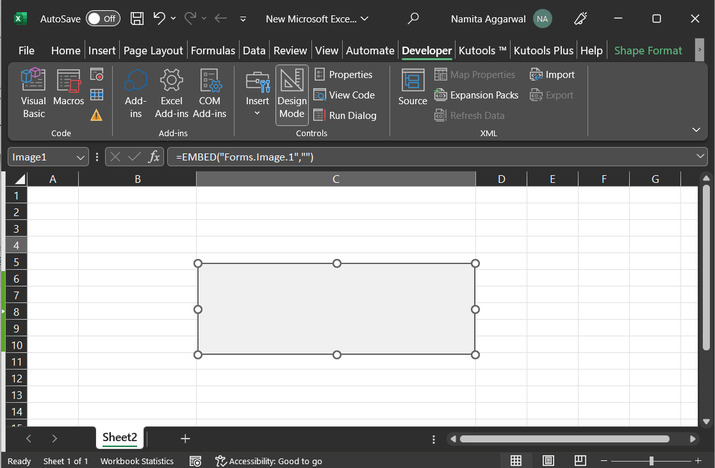
This step will provide a draw cursor, drag the cursor and draw a rectangular shape, at any required location. The drawn triangle is shown below for reference:
Step 3
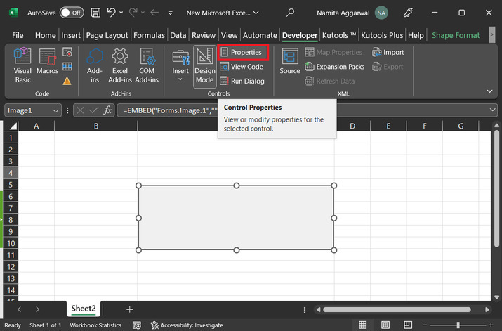
After that select the drawing pattern and go to the Developer tab, again, and under the controls option, click on the "Properties" button. For reference consider the below provided snapshot of data:
Step 4
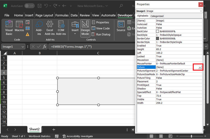
The above step will display a "Properties" dialog box. This dialog box shows different options. This dialog box contains two tabs alphabetic and categorized. For this example, will choose the second tab, and click on the "Picture" option, after that click on the three?dotted line provided in the front of the pictures tab.
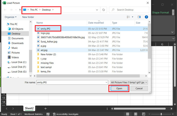
Step 5
The above step will open a "Load Picture" dialog box. In the load picture dialog box, browse the jpg file user wants to insert into the Excel sheet. Here, the name of the used image is "smily.jpg", and it is available at the desktop location. Finally, click on the "OK" button.
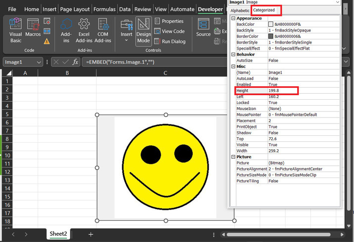
Step 6
The inserted image will now see inside the created image control. Users can also change the height of the inserted image according to requirements. For example, here will be modifying the sheet height to 199.8, by clicking on the height button. snapshot for the same is provided below:
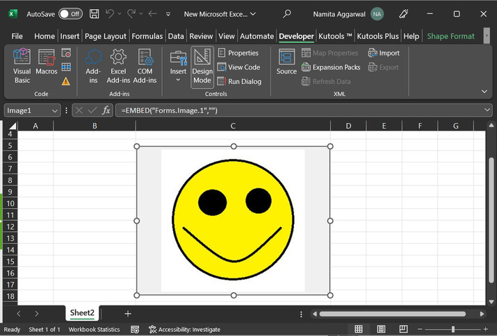
Step 7
The final inserted image control is provided below. Users can adjust the height and width of the image according to their requirements. For the taken sample the possible image is depicted below:
Conclusion
This article illustrates an example to insert the image control in an Excel file. By using the guided steps accurately user can learn the process of inserting the image control in Excel. The user should save the image to a proper location, before importing it to the Excel sheet.

709 Views
