How to identify and return row and column number of cell in Excel?

In this article, the user will learn how to identify and return row and columns number of cells in Excel to process some important data. This article provided two examples to illustrate the way to identify the row and column numbers from the provided Excel data. In the first example, the user must complete the address of the Excel sheet and needs to calculate the separate row and column values for the cells. Examples include the use of predefined row () and column () and match () formula methods to calculate the respective row() and column() values.

Example 1: To obtain the column and row number when the user knows the complete address.

Step 1

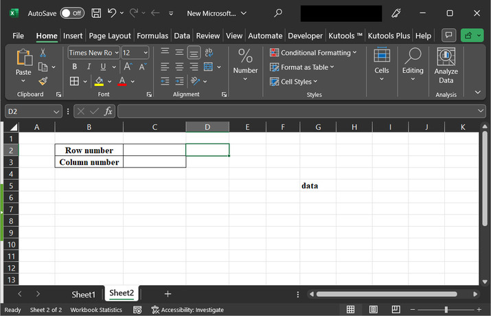
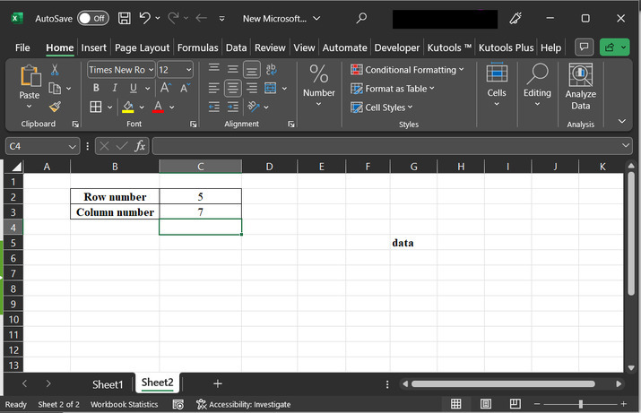
In this example, the user will learn the process to extract the row and column. The considered Excel sheet contains two cell headers: first for row number at B2 cell, and second for column number B3. A snapshot for reference is provided below:

Step 2

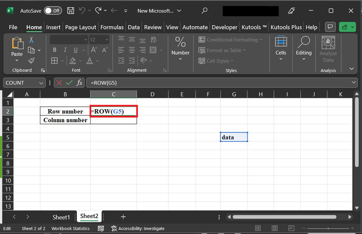
Go to the C2 cell, and type the formula “=Row(G5)”. This formula will allow the user to evaluate the associated row number from the cell. A snapshot for reference is provided below:

Step 3

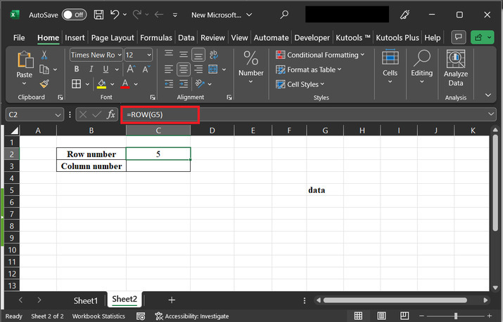
Press the “Enter key” to display the calculated result data on the sheet. The generated row number is 5th this means that the data is present on the 5 th row of the provided spreadsheet.

Step 4

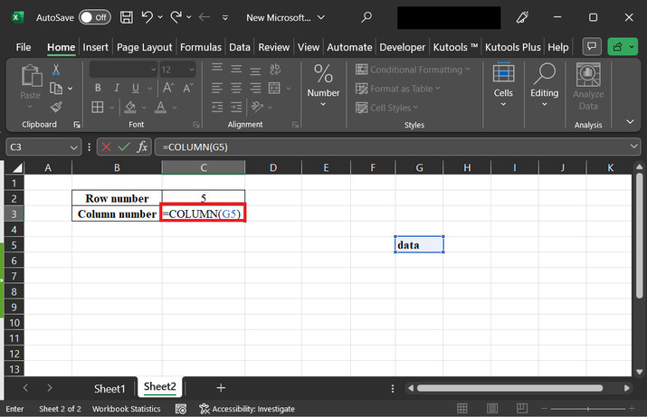
This step will try to obtain the column value of the cell that contains address G5. Go to the C3 cell, and type the formula “=Column(G5)”. A snapshot for the same is depicted below:

Step 5

Press the enter key to obtain the required column value. Snapshot for reference is provided below:

Example 2: To obtain the column and row number by using the match formula.

Step 1

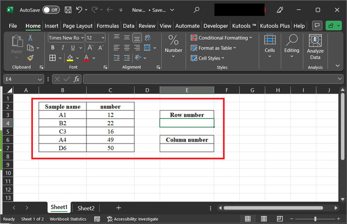
Using match() function to calculate the required row and column values. To do so, assume that the spreadsheet contains “sample name”, and “number”. Go to the E3 cell to create a cell header for the “row number”, and E6 cell to create a column header. A snapshot for reference is provided below:

Step 2

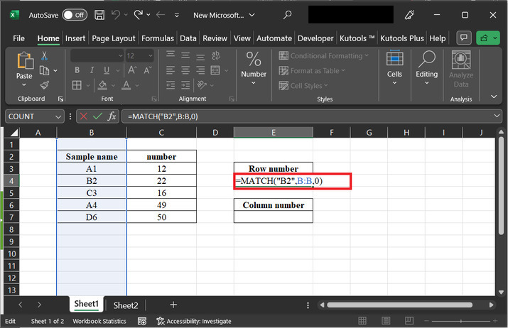
In this step, select the sample name column, then go to the E4 cell, and type the formula. “=MATCH("B2",B:B,0)”

Explanation

• The provided formula contains an equal sign this shows that the first argument is B2. "B2" with a value equal to "B:B" as a second argument. The second argument is a column reference for the sheet, it represents the data user needs to search within the column., which represents the range of cells we want to search within (the entire column B). The third argument, 0, specifies that we want an exact match.

Step 3

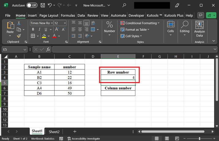
Press the “Enter” key to display the required result on the Excel sheet. A snapshot for reference is provided below:

Step 4

After that go to the E7 cell, and type formula “=MATCH("B2",4:4,0)” to the cell. A snapshot for reference is provided below:

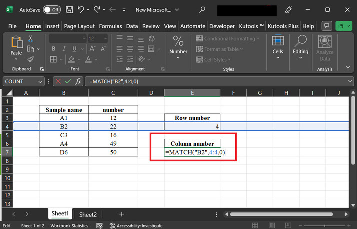
Explanation for formula

• In the above formula, "B2" is a Lookup_value. It represents a value or cell reference that the user wants to determine within the range.

• After that go to the Lookup_array which is 4:4. That is the range of available data cells in which you want to search for the lookup_value. In this case, it refers to row 4.

• After that, the next provided value is 0, which means that the match type value is 0. This parameter specifies the type of match the user wants to perform.

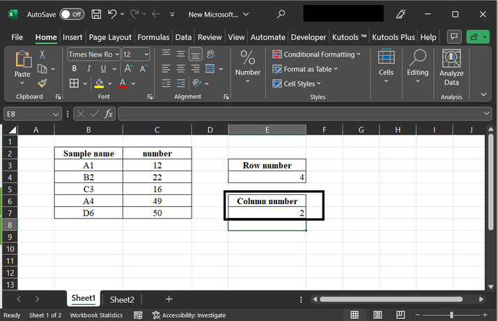
Step 5

Press the “Enter” key, to view the generated results. A snapshot of the result is provided below:

Conclusion

This article contains illustrations for two examples, both examples are accurate are precise, and the explanations provided for all the steps are detailed and thorough. By following all the guided steps proper user can easily perform the required task.