
Article Categories
- All Categories
-
 Data Structure
-
 Networking
-
 RDBMS
RDBMS
-
 Operating System
-
 Java
Java
-
 MS Excel
-
 iOS
iOS
-
 HTML
HTML
-
 CSS
CSS
-
 Android
-
 Python
-
 C Programming
-
 C++
C++
-
 C#
C#
-
 MongoDB
-
 MySQL
MySQL
-
 Javascript
-
 PHP
PHP
-
 Economics & Finance
How to get row or column letter of the current cell in Excel?
Excel spreadsheet store data in table format. Every Excel sheet is made up of rows and columns. Rows are the horizontal record fields available in the Excel sheet. On the other hand, columns are the vertical record fields available in the Excel sheet. Row address values are represented by using numbers. While column data values will be represented by using the alphabet. Since row data is represented by using numbers, therefore, they are required to be get converted into an alphabet value. While column data is already available in the form of letters.
Example 1: To get row letter in Excel by using the predefined formula:
Step 1:
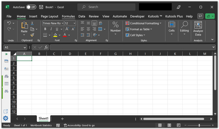
Consider a blank Excel sheet. This blank sheet contains an active cell A1. In this example, the user will try to obtain the row number, and after that convert the obtained row number to letter, by using the available predefined methods of Excel.
Step 2:
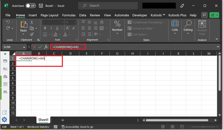
After that go to the A2 cell, and type formula "=CHAR(ROW()+64)".
An explanation for the above mentioned formula:
The above-provided function will return an uppercase letter that corresponds to the current row number of the cell where the user has entered the formula.
The "+64" part of the formula is used to offset the ASCII code value. So, that the function returns the correct letter. The ASCII code for the letter "A" is 65, so by adding 64, the formula returns the correct letter for the corresponding row number.
For this case, the formula is entered in the A1 cell. This function will return "A".
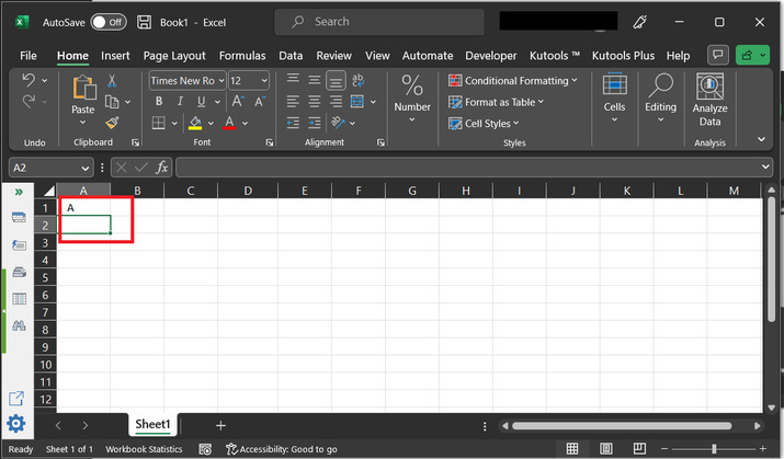
Step 3:
After that press the "Enter" key. This will display "A", to the A1 cell.
Example 2: To get column letters in Excel by using the predefined formula:
Step 1:
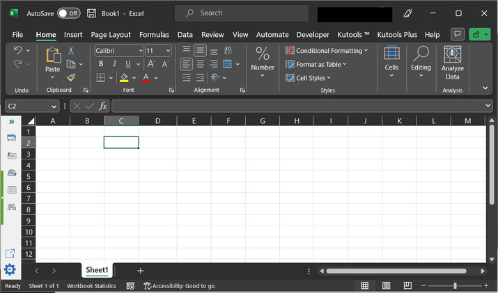
Consider a blank Excel sheet. This blank sheet contains an active C2 cell. In this example, the user will try to obtain the column number, and display the column letter by using the available predefined methods of Excel.
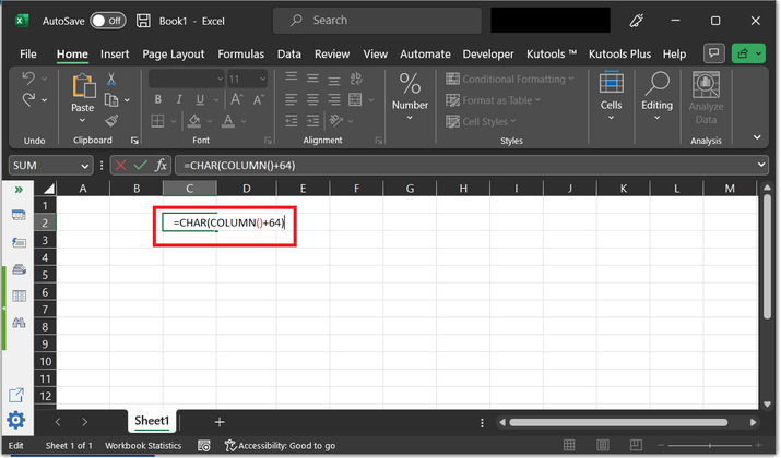
Step 2:
After that go to the C2 cell, and type formula "=CHAR(COLUMN()+64)".
Explanation for the above-mentioned formula:
The above provided formula will return the uppercase letter that is relevant to the current column number of the cell where the formula is entered.
The "+64" part of the formula is used to offset the ASCII code value. So, that the function returns the correct letter. The ASCII code for the letter "A" is 65, so by adding 64, the formula returns the correct letter for the corresponding column number.
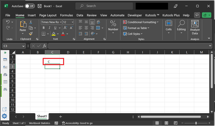
For this case, the formula is entered in the C2 cell. This function will return "C".
Step 3:
After that press the "Enter" key. This will display the "C" associated column name to the A1 cell.
Conclusion:
This article contains two examples to obtain the row and column letters of the active cell. Both the provided examples are using predefined formulas. The used method names are ROW() and COLUMN(). The ROW() method returns the row data value. COLUMN() method returns the column data value.

5K+ Views
