How To Create Dynamic Cascading List Boxes In Excel?

Excel is a powerful tool for data analysis and manipulation. One of its features is the ability to create dynamic cascading list boxes, which allows users to select items from a dropdown list based on a previous selection. This can be especially useful for organizing and filtering large amounts of data.

In this tutorial, we will explore how to create dynamic cascading list boxes in Excel. We will start by discussing the concept of cascading list boxes and their benefits, and then move on to the step-by-step process of creating them in Excel. We will also cover some tips and tricks to help you customize and optimize your cascading list boxes. By the end of this tutorial, you will have a thorough understanding of how to create dynamic cascading list boxes in Excel and how to apply them to your data analysis tasks. So, let's get started!

Create Dynamic Cascading List Boxes

Here we will first list the unique values, modify the properties of the ActiveX controls list box, and finally use the VAB code to complete the task. So let us see a simple process to know how you can create dynamic cascading list boxes in Excel.

Step 1

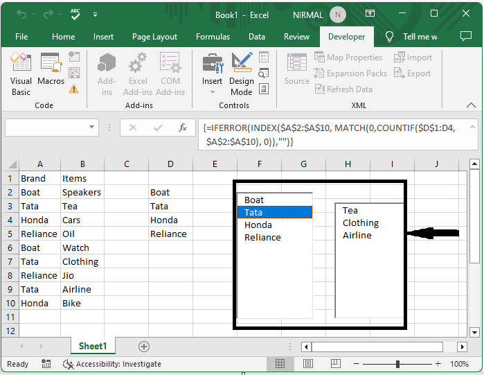
Consider an Excel sheet where the data is similar to the below image.

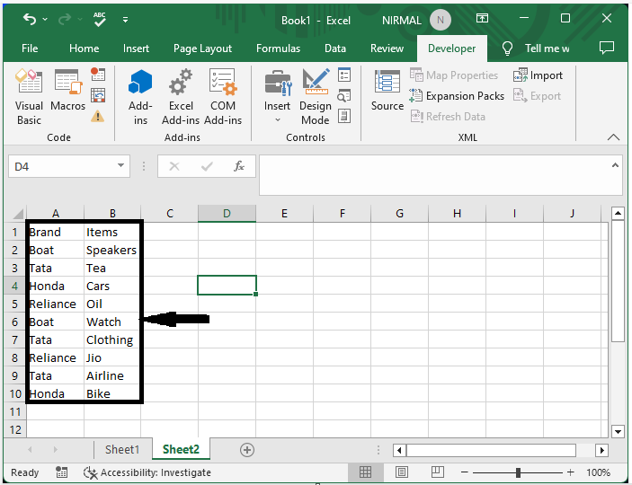
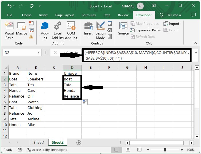
First click on an empty cell in our case cell D2 and enter the formula as

=IFERROR(INDEX($A$2:$A$10, MATCH(0,COUNTIF($D$1:D1, $A$2:$A$10), 0)),"") and click CTRL + SHIFT + ENTER to get the first value and drag down using the auto-fill handle to get all the unique records.

Empty cell > Formula > CTRL + SHIFT + ENTER > Drag.

Step 2

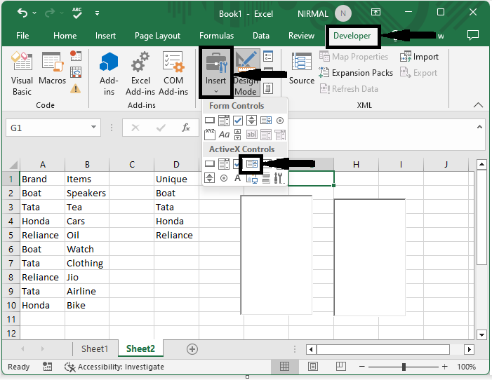
Now click on Developer, then insert, and draw two list boxes from ActiveX controls.

Developer > Insert > List box > Draw.

Step 3

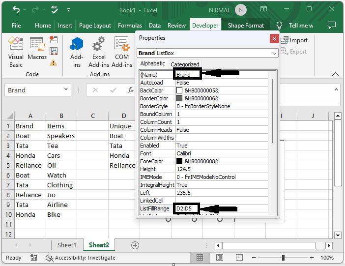
Then right-click on the first box and select properties, then set name as Brand and listfillrange to D2:D5 (range of unique values).

Right click > Properties > Name > Listfillrange.

Step 4

Again, right-click on the second list and set the name to Items.

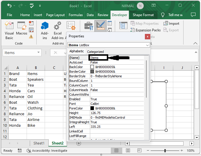
Step 5

Then right-click on the sheet name and select View code to open the VBA application, and copy the below-mentioned code into the text box

Right click > View code > Copy code

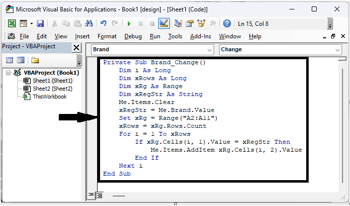
Code

Private Sub Brand_Change()
   Dim i As Long
   Dim xRows As Long
   Dim xRg As Range
   Dim xRegStr As String
   Me.Items.Clear
   xRegStr = Me.Brand.Value
   Set xRg = Range("A2:A11")
   xRows = xRg.Rows.Count
   For i = 1 To xRows
      If xRg.Cells(i, 1).Value = xRegStr Then
         Me.Items.AddItem xRg.Cells(i, 2).Value
      End If
   Next i
End Sub

Step 6

Then close the VBA application and turn off the design mode, and our final output will be similar to the below image.

Conclusion

In this tutorial, we have used a simple example to demonstrate how you can create dynamic cascading list boxes in Excel to highlight a particular set of data.