- Cosmology - Home
- The Expanding Universe
- Cepheid Variables
- Redshift and Recessional Velocity
- Redshift Vs. Kinematic Doppler Shift
- Cosmological Metric & Expansion
- Robertson-Walker Metric
- Hubble Parameter & Scale Factor
- Friedmann Equation & World Models
- Fluid Equation
- Matter Dominated Universe
- Radiation Dominated Universe
- The Dark Energy
- Spiral Galaxy Rotation Curves
- Velocity Dispersion Measurements of Galaxies
- Hubble & Density Parameter
- Age of The Universe
- Angular Diameter Distance
- Luminosity Distance
- Type 1A Supernovae
- Cosmic Microwave Background
- CMB - Temperature at Decoupling
- Anisotropy of CMB Radiation & Cobe
- Modelling the CMB Anisotropies
- Horizon Length at the Surface of Last Scattering
- Extrasolar Planet Detection
- Radial Velocity Method
- Transit Method
- Exoplanet Properties
Cosmology - Quick Guide
Cosmology - The Expanding Universe
Cosmology is the study of the universe. Tracing back in the time, there were several school of thoughts regarding the origin of the universe. Many scholars believed in the Steady State Theory. As per this theory, the universe was always the same, it had no beginning.
While there were a group of people who had faith in the Big Bang Theory. This theory predicts the beginning of the universe. There were evidences of hot left out radiation from the Big Bang, which again supports the model. The Big Bang Theory predicts the abundance of light elements in the universe. Thus, following the famous model of Big Bang, we can state that the universe had a beginning. We are living in an expanding universe.
The Hubble Redshift
In the early 1900s, the state of the art telescope, Mt Wilson, a 100-inch telescope, was the biggest telescope then. Hubble was one of the prominent scientists, who worked with that telescope. He discovered there were galaxies outside the Milky Way. Extragalactic Astronomy is only 100 years old. Mt Wilson was the biggest telescope until Palmer Observatory was built which had a 200-inch telescope.
Hubble was not the only person observing galaxies outside the Milky Way, Humason helped him. They set out on measuring the spectra of nearby galaxies. They then observed a galactic spectrum was in the visible wavelength range with continuous emission. There were emission and absorption lines on top of the continuum. From these lines, we can make an estimate if the galaxy is moving away from us or towards us.
When we get a spectrum, we assume the strongest line is coming from H-α. From literature, the strongest line should occur at 6563 Å, but if the line occurs somewhere around 7000Å, we can easily say it is redshifted.
From the Special Theory of Relativity,
$$1 + z = \sqrt{\frac{1+\frac{v}{c}}{1-\frac{v}{c}}}$$
where, Z is the redshift, a dimensionless number and v is the recession velocity.
$$\frac{\lambda_{obs}}{\lambda_{rest}} = 1 + z$$
Hubble and Humason listed down 22 Galaxies in their paper. Nearly all these galaxies exhibited redshift. They plotted the velocity (km/s) vs distance (Mpc). They observed a linear trend and Hubble put forward his famous law as follows.
$$v_r = H_o d$$
This is the Hubble Redshift Distance Relationship. The subscript r indicates expansion is in the radial direction. While, $v_r$ is the receding velocity, $H_o$ is the Hubble parameter, d is the distance of the galaxy from us. They concluded far away galaxies recede faster from us, if the rate of expansion for the universe is uniform.
The Expansion
Everything is moving away from us. The galaxies are not stationary, there is some expansion harmonic always. The units of the Hubble parameter are km sec1Mpc1. If one goes out a distance of 1 Mpc, galaxies would be moving at the rate of 200 kms/sec. The Hubble parameter gives us the rate of expansion. As per Hubble and Humason, the value of $H_o$ is 200 kms/sec/Mpc.
The data showed all galaxies are moving away from us. Thus, it is apparent that we are at the center of the universe. But Hubble didnt make this mistake, as per him, in whichever galaxy we live, we would find all other galaxies moving away from us. Thus, the conclusion is that the space between galaxies expand and there is no center of the universe.
The expansion is happening everywhere. However, there are some forces that are opposing expansion. Chemical bonds, gravitational force and other attractive forces are holding objects together. Earlier all the objects were close together. Considering the Big Bang as an impulsive force, these objects are set to move away from each other.
Time Scale
At local scales, Kinematics is governed by Gravity. In the original Hubbles law, there were some galaxies which showed blue-shift. This can be credited to combined gravitational potential of the galaxies. Gravity has decoupled things from the Hubbles law. The Andromeda Galaxy is coming towards to us. Gravity is trying to slow things down. Initially the expansion was slowing down, now it is speeding up.
There was a Cosmic Jerk because of this. Several estimates to the Hubble parameter has been made. It has evolved over the 90 years from 500 kms/sec/Mpc to 69 kms/sec/Mpc. The disparity in the value was because of the underestimation of distance. The Cepheid Stars were used as distance calibrators, however there are different types of Cepheid stars and this fact was not considered for the estimation of the Hubble parameter.
Hubble Time
The Hubble constant gives us a realistic estimate of the age of the universe. The $H_o$ would give the age of the universe provided the galaxies have been moving with the same velocity. The inverse of $H_o$ gives us Hubble time.
$$t_H = \frac{1}{H_o}$$
Replacing the present value of $H_o, t_H$ = 14 billion years. Rate of expansion has been constant throughout the beginning of the Universe. Even if this is not true, $H_o$ gives a useful limit on the age of the universe. Assuming a constant rate of expansion, when we plot a graph between distance and time, the slope of the graph is given by velocity.
In this case, the Hubble time is equal to the actual time. However, if the universe had been expanding faster in the past and slower in the present, the Hubble time gives an upper limit of age of the universe. If the universe was expanding slowly before, and speeding up now, then the Hubble time will give a lower limit on age of the universe.
$t_H = t_{age}$ − if rate of expansion is constant.
$t_H > t_{age}$ − if universe has expanded faster in the past and slower in the present.
$t_H < t_{age}$ − if universe has expanded slower in the past and faster in the present.
Consider a group of 10 galaxies which are at 200 Mpc from another group of galaxies. The galaxies within a cluster never conclude that the universe is expanding because kinematics within a local group is governed by gravitation.
Points to Remember
Cosmology is the study of the past, present and future of our Universe.
Our universe is ∼14 billion years old.
The universe is continuously expanding.
Hubble parameter is a measure of the age of the universe.
Current value of Ho is 69 kms/sec/Mpc.
Cosmology - Cepheid Variables
For a very long time, nobody considered galaxies to be present outside our Milky Way. In 1924, Edwin Hubble detected Cepheids in the Andromeda Nebula and estimated their distance. He concluded that these "Spiral Nebulae" were in fact other galaxies and not a part of our Milky Way. Hence, he established that M31 (Andromeda Galaxy) is an Island Universe. This was the birth of Extragalactic Astronomy.
Cepheids show a periodic dip in their brightness. Observations show that the period between successive dips called the period of pulsations is related to luminosity. So, they can be used as distance indicators. The main sequence stars like the Sun are in Hydrostatic Equilibrium and they burn hydrogen in their core. After hydrogen is fully burned, the stars move towards the Red Giant phase and try to regain their equilibrium.
Cepheid Stars are post Main Sequence stars that are transiting from the Main Sequence stars to the Red Giants.
Classification of Cepheids
There are 3 broad classes of these pulsating variable stars −
Type-I Cepheids (or Classical Cepheids) − period of 30-100 days.
Type-II Cepheids (or W Virginis Stars) − period of 1-50 days.
RR Lyrae Stars − period of 0.1-1 day.
At that time, Hubble was not aware of this classification of variable stars. That is why there was an overestimation of the Hubble constant, because of which he estimated a lower age of our universe. So, the recession velocity was also overestimated. In Cepheids, the disturbances propagate radially outward from the centre of the star till the new equilibrium is attained.
Relation between Brightness and Pulsation Period
Let us now try to understand the physical basis of the fact that higher pulsation period implies more brightness. Consider a star of luminosity L and mass M.
We know that −
$$L \propto M^\alpha$$
where α = 3 to 4 for low mass stars.
From the Stefan Boltzmann Law, we know that −
$$L \propto R^2 T^4$$
If R is the radius and $c_s$ is the speed of sound, then the period of pulsation P can be written as −
$$P = R/c_s$$
But the speed of sound through any medium can be expressed in terms of temperature as −
$$c_s = \sqrt{\frac{\gamma P}{\rho}}$$
Here, γ is 1 for isothermal cases.
For an ideal gas, P = nkT, where k is the Boltzmann Constant. So, we can write −
$$P = \frac{\rho kT}{m}$$
where $\rho$ is the density and m is the mass of a proton.
Therefore, period is given by −
$$P \cong \frac{Rm^{\frac{1}{2}}}{(kT)^{{\frac{1}{2}}}}$$
Virial Theorem states that for a stable, self-gravitating, spherical distribution of equal mass objects (like stars, galaxies), the total kinetic energy k of the object is equal to minus half the total gravitational potential energy u, i.e.,
$$u = -2k$$
Let us assume that virial theorem holds true for these variable stars. If we consider a proton right on the surface of the star, then from the virial theorem we can say −
$$\frac{GMm}{R} = mv^2$$
From Maxwell distribution,
$$v = \sqrt{\frac{3kT}{2}}$$
Therefore, period −
$$P \sim \frac{RR^{\frac{1}{2}}}{(GM)^{\frac{1}{2}}}$$
which implies
$$P \propto \frac{R^{\frac{3}{2}}}{M^{\frac{1}{2}}}$$
We know that $M \propto L^{1/\alpha}$
Also $R \propto L^{1/2}$
So, for β > 0, we finally get $P \propto L^\beta$
Points to Remember
Cepheid Stars are post Main Sequence stars that are transiting from the Main Sequence stars to Red Giants.
Cepheids are of 3 types: Type-I, Type-II, RR-Lyrae in decreasing order of pulsating period.
Pulsating period of Cepheid is directly proportional to its brightness (luminosity).
Redshift and Recessional Velocity
Hubbles observations made use of the fact that radial velocity is related to shifting of the Spectral Lines. Here, we will observe four cases and find a relationship between Recessional Velocity ($v_r$) and Red Shift (z).
Case 1: Non-Relativistic Case of Source moving
In this case, v is much less than c. Source is emitting some signal (sound, light, etc.), which is propagating as Wavefronts. The time interval between the sending of two consecutive signals in the source frame is Δts. The time interval between the reception of two consecutive signals in the observer frame is Δto.
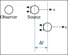
If both the observer and source are stationary, then Δts = Δto, but this is not the case here. Instead, the relation is as follows.
$$\Delta t_o = \Delta t_s + \frac{\Delta l}{c}$$
Now, $\Delta l = v \Delta t_s$
Also, since (wave speed x time) = wavelength, we get
$$\frac{\Delta t_o}{\Delta t_s} = \frac{\lambda_o}{\lambda_s}$$
From the above equations, we get the following relation −
$$\frac{\lambda_o}{\lambda_s} = 1 + \frac{v}{c}$$
where $\lambda _s$ is the wavelength of the signal at the source and $\lambda _o$ is the wavelength of the signal as interpreted by the observer.
Here, since the source is moving away from the observer, v is positive.
Red shift −
$$z = \frac{\lambda_o - \lambda_s}{\lambda_s} = \frac{\lambda_o}{\lambda_s} - 1$$
From the above equations, we get Red shift as follows.
$$z = \frac{v}{c}$$
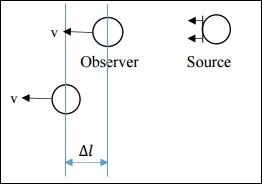
Case 2: Non-Relativistic Case of Observer Moving
In this case, v is much less than c. Here, $\Delta l$ is different.
$$\Delta l = v \Delta t_o$$
On simplification, we get −
$$\frac{\Delta t_o}{\Delta t_s} = \left ( 1 - \frac{v}{c} \right )^{-1}$$
We get Red shift as follows −
$$z = \frac{v/c}{1-v/c}$$
Since v << c, the red shift expression for both Case I and Case II are approximately the same.
Let us see how the red shifts obtained in the above two cases differ.
$$z_{II} - z_I = \frac{v}{c} \left [ \frac{1}{1 - v/c}-1 \right ]$$
Hence, $z_{II} z_{I}$ is a very small number due to the $(v/c)^2$ factor.
This implies that, if v << c, we cannot tell whether the source is moving, or the observer is moving.
Let us now understand the Basics of STR (Special Theory of Relativity) −
Speed of light is a constant.
When the source (or observer) is moving with a speed comparable to the speed of light, relativistic effects are observed.
Time dilation: $\Delta t_o = \gamma \Delta t_s$
Length contraction: $\Delta l_o = \Delta t_s/\gamma$
Here, $\gamma$ is the Lorrentz factor, greater than 1.
$$\gamma = \frac{1}{\sqrt{1-(v^2/c^2)}}$$
Case 3: Relativistic Case of Source Moving
In this case, v is comparable to c. Refer to the same figure as in Case I. Due to the relativistic effect, time dilation is observed and hence the following relation is obtained. (Source is moving with relativistic speed)
$$\Delta t_o = \gamma \Delta t_s + \frac{\Delta l}{c}$$
$$\Delta l = \frac{v\gamma \Delta t_s}{c}$$
$$\frac{\Delta t_o}{\Delta t_s} = \frac{1 + v/c}{\sqrt{1- (v^2/c^2)}}$$
On further simplification, we get,
$$1 + z = \sqrt{\frac{1+v/c}{1-v/c}}$$
The above expression is known as the Kinematic Doppler Shift Expression.
Case 4: Relativistic Case of Observer Moving
Refer to the same figure as in Case II. Due to relativistic effect, time shortening is observed and hence the following relation is obtained. (Observer is moving with relativistic speed)
$$\Delta t_o = \frac{\Delta t_s}{\gamma}+\frac{\Delta l}{c}$$
$$\Delta l = \frac{v\Delta t_o}{c}$$
$$\frac{\Delta t_o}{\Delta t_s} = \frac{\sqrt{1-( v^2/c^2)}}{1-v/c}$$
On further simplification, we get −
$$1 + z = \sqrt{\frac{1+ v/c}{1- v/c}}$$
The above expression is the same as what we got for Case III.
Points to Remember
Recessional velocity and redshift of a star are related quantities.
In a non-relativistic case, we cannot determine whether the source is moving or stationary.
In a relativistic case, there is no difference in the redshift-recessional velocity relationship for source or observer moving.
Moving clocks move slower, is a direct result of relativity theory.
Redshift Vs. Kinematic Doppler Shift
A galaxy which is at redshift z = 10, corresponds to v≈80% of c. The mass of the Milky Way is around 1011M⊙, if we consider the dark matter, it is 1012M⊙. Our milky way is thus massive. If it moves at 80% of c, it does not fit in the general concept of how objects move.
We know,
$$\frac{v_r}{c} = \frac{\lambda_{obs} - \lambda{rest}}{\lambda_{rest}}$$
For small values of z,
$$z = \frac{v_r}{c} = \frac{\lambda_{obs}-\lambda_{rest}}{\lambda_{rest}}$$
In the following graph, the class between flux and wavelength, there are emission lines on top of the continuum. From the H-α line information, we get to conclude that roughly z = 7. This implies galaxy is moving at 70% of c. We are observing a shift and interpreting it as velocity. We should get rid of this notion and look at z in a different way. Imagine space as a 2D grid representing the universe as shown below.
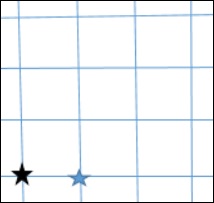
Consider the black star to be our own milky way and the blue star to be some other galaxy. When we record light from this galaxy, we see the spectrum and find out its redshift i.e., the galaxy is moving away. When the photon was emitted, it had relative velocity.
What if the space was expanding?
It is an instantaneous redshift of photon. Cumulative redshifts along the space between two galaxies will tend to a large redshift. The wavelength will change finally. It is the expansion of the space rather than the kinematic movement of the galaxies.
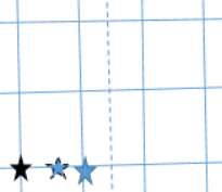
The following image shows if mutual gravity overflows expansion then this is not participating in the Hubbles law.
In the Kinematic Doppler Shift, the redshift is induced in a photon at the time of emission. In a Cosmological Redshift, in every step, it is getting cumulatively redshifted. In a gravitational potential, a photon will get blue shifted. As it crawls out of gravitational potential, it gets redshifted.
As per a Special Theory of Relativity, two objects passing by each other cannot have a relative velocity greater than the speed of light. The velocity we speak about is of the expansion of the universe. For large values of z, the redshift is cosmological and not a valid measure of the actual recessional velocity of the object with respect to us.
The Cosmological Principle
It stems from the Copernicus Notion of the universe. As per this notion, the universe is homogeneous and isotropic. There is no preferred direction and location in the universe.
Homogeneity means no matter which part of the universe you reside in, you will see universe is the same in all parts. Isotropic nature means no matter which direction you look, you are going to see the same structure.
A fitting example of homogeneity is a Paddy field. It looks homogeneous from all parts, but when wind flows, there are variations in its orientation, thus it is not isotropic. Consider a mountain on a flat land and an observer is standing on the mountain top. He will see the isotropic nature of the flat land, but it is not homogeneous. If in a homogeneous universe, it is isotropic at a point, it is isotropic everywhere.
There have been large scale surveys to map the universe. Sloan Digital Sky Survey is one such survey, which did not focus much on the declination, but on the right ascension. The lookback time is around 2 billion years. Every pixel corresponds to the location of a galaxy and the color corresponds to the morphological structure. The green color represented blue spiral galaxy while the red false color indicated massive galaxies.
Galaxies are there in a filamentary structure in a cosmological web and there are voids in between the galaxies.
$\delta M/M \cong 1$ i.e., fluctuation of mass distribution is 1 M is the mass of the matter present within a given cube. In this case, take the volume 50 Mpc cube.
For a cube side of 1000 Mpc, $\delta M/M \cong 10^{4}$.
One way to quantify homogeneity is to take mass fluctuations. Mass fluctuations will be higher at lower scales.
For quantifying the isotropic nature, consider cosmic microwave background radiation. Universe is nearly isotropic at large angular scales.
Points to Remember
Two objects passing by each other cannot have a relative velocity greater than the speed of light.
Cosmological Principle states that the universe is homogeneous and isotropic.
This homogeneity exists at a very large angular scale and not on smaller scales.
SDSS (Sloan Digital Sky Survey) is an effort to map the night sky, verifying the Cosmological Principle.
Cosmological Metric & Expansion
As per the law of conservation of energy and the law of conservation of mass, the total amount of energy including the mass (E=mc2) remains unchanged throughout every step in any process in the universe. The expansion of the universe itself consumes energy which maybe from the stretching of wavelength of photons (Cosmological Redshift), Dark Energy Interactions, etc.
To speed up the survey of more than 26,000 galaxies, Stephen A. Shectman designed an instrument capable of measuring 112 galaxies simultaneously. In a metal plate, holes that corresponded to the positions of the galaxies in the sky were drilled. Fiber-optic cables carried the light from each galaxy down to a separate channel on a spectrograph at the 2.5-meter du Pont telescope at the Carnegie Observatories on Cerro Las Campanas in Chile.
For maximum efficiency, a specialized technique known as the Drift-Scan Photometry was used, in which the telescope was pointed at the beginning of a survey field and then automated drive was turned off. The telescope stood still as the sky drifted past. Computers read information from the CCD Detector at the same rate as the rotation of the earth, producing one long, continuous image at a constant celestial latitude. Completing the photometry took a total of 450 hours.
Different forms of noise exist and their mathematical modelling is different depending upon its properties. Various physical processes evolve the power spectrum of the universe on a large scale. The initial power spectrum imparted due to the quantum fluctuations follows a negative third power of frequency which is a form of Pink Noise Spectrum in three dimensions.
The Metric
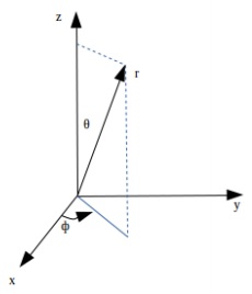
In cosmology, one must first have a definition of space. A metric is a mathematical expression describing points in space. The observation of the sky is done in a spherical geometry; hence a spherical coordinate system shall be used. The distance between two closely spaced points is given by −
$$ds^2 = dr^2 + r^2\theta ^2 + r^2 sin^2\theta d\phi^2$$
The following image shows Geometry in the 3-dimensional non-expanding Euclidean space.
This geometry is still in the 3-dimensional non-expanding Euclidean space. Hence, the reference grid defining the frame itself would be expanding. The following image depicts the increased metric.
A scale factor is put into the equation of the non-expanding space, called the scale factor which incorporates expansion of the universe with respect to time.
$$ds^2 = a^2(t)\left [ dr^2 + r^2\theta^2 + r^2 sin^2\theta d\phi^2 \right ]$$
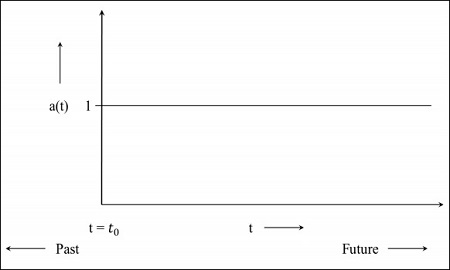
where a(t) is the scale factor, sometimes written as R(t). Whereas, a(t) > 1 means magnification of the metric, while a(t) < 1 means shrinking of the metric and a(t) = 1 means constant metric. As a convention, a(t0) = 1.
Comoving Coordinate System
In a Comoving Coordinate System, the measuring scale expands along with the frame (expanding universe).
Here, the $\left [ dr^2 + r^2\theta^2 + r^2 sin^2\theta d\phi^2 \right ]$ is the Comoving Distance, and the $ds^2$ is the Proper distance.
The proper distance will correspond to the actual distance as measured of a distant galaxy from earth at the time of observation, a.k.a. instantaneous distance of objects.
This is because the distance travelled by a photon when it reaches the observer from a distant source will be the one received at $t=t_0$ of the observer, which would mean that the instantaneous observed distance will be the proper distance, and one can predict future distances using the rate factor and the initial measured length as a reference.
The concept of Comoving and proper distance is important in measuring the actual value of the number density of galaxies in the given volume of the observed space. One must use the Comoving distance to calculate the density at the time of their formation when the observed photon was emitted. That can be obtained once the rate of expansion of the universe can be estimated.
To estimate the rate of expansion, one can observe the change in the distance of an observed distant galaxy over a long period of time.
Points to Remember
A metric is a mathematical expression describing the points in space.
The scale factor determines whether the universe is contracting or expanding.
In a comoving coordinate system, the measuring scale expands along with the frame (expanding universe).
Proper distance is the instantaneous distance of objects.
Comoving distance is the actual distance of objects.
Cosmology - Robertson-Walker Metric
In this chapter, we will understand in detail regarding the Robertson-Walker Metric.
Model for Scale Factor Changing with Time
Suppose a photon is emitted from a distant galaxy. The space is forward for photon in all directions. The expansion of the universe is in all the directions. Let us see how the scale factor changes with time in the following steps.
Step 1 − For a static universe, the scale factor is 1, i.e. the value of comoving distance is the distance between the objects.
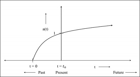
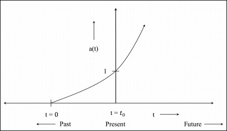
Step 2 − The following image is the graph of the universe that is still expanding but at a diminishing rate, which means the graph will start in the past. The t = 0 indicates that the universe started from that point.
Step 3 − The following image is the graph for the universe which is expanding at a faster rate.
Step 4 − The following image is the graph for the universe that starts contracting from now.
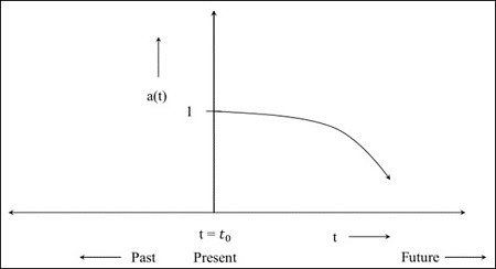
If the value of the scale factor becomes 0 during the contraction of universe, it implies the distance between the objects becomes 0, i.e. the proper distance becomes 0. The comoving distance which is the distance between the objects at a present universe, is a constant quantity. In the future, when the scale factor becomes 0, everything will come closer. The model depends on the component of the universe.
The Metric for flat (Euclidean: there is no parameter for curvature) expanding universe is given as −
$$ds^2 = a^2(t)\left ( dr^2+r^2d\theta^2+r^2sin^2\theta d\varphi^2 \right )$$
For spacetime, the line element that we obtained in the above equation is modified as −
$$ds^2 = c^2dt^2 - \left \{ a^2(t) \left ( dr^2 + r^2d\theta ^2 + r^2sin^2\theta d\varphi^2 \right ) \right \}$$
For space time, the time at which the photon is emitted and when it is detected is different. The proper distance is the instantaneous distance to objects which can change over time due to the expansion of the universe. It is the distance that the photon had travelled from different objects to get to us. It is related to the comoving distance as −
$$d_p = a(t) \times d_c$$
where $d_p$ is the proper distance and $d_c$ is the comoving distance, which is fixed.
The distance measured to the objects in the present universe is taken as the comoving distance, which means the comoving distance is fixed and is unchanged by the expansion. For past, the scale factor was less than 1, which indicates that the proper distance was smaller.
We can measure the redshift to a galaxy. Hence the proper distance $d_p$ corresponds to $c \times t(z)$, where $t(z)$ is the lookback time towards a redshift and c is the speed of light in vacuum. The lookback time is a function of the redshift (z).
Based on the above notion, let us analyze how cosmological red shift is interpreted in this scenario of $d_p = a(t) \times d_c$.
Assume a photon (which is earth bound) is emitted by the galaxy, G. The $t_{em}$ corresponds to the time when photon was emitted; $a(t_{em})$ was the scale factor at that time when the photon was emitted. By the time of detection of the photon, the whole universe had expanded, i.e. the photon is redshifted at the time of detection. The $t_{obs}$ corresponds to the time when the photon is detected and the corresponding scale factor is $a(t_{obs})$.
The factor by which the universe has grown is given by −
$$\frac{a(t_{obs})}{a(t_{em})}$$
The factor by which wavelength has expanded is −
$$\frac{\lambda_{obs}}{\lambda_{em}}$$
which is equal to the factor by which the universe has grown. The symbols have their usual meaning. Therefore,
$$\frac{a(t_{obs})}{a(t_{em})} = \frac{\lambda_{obs}}{\lambda_{em}}$$
We know that redshift (z) is −
$$z=\frac{\lambda_{obs} - \lambda_{em}}{\lambda_{em}} = \frac{\lambda_{obs}}{\lambda_{em}} - 1$$
$$1 + z = \frac{a(t_{obs})}{a(t_{em})}$$
The present value of the scale factor is 1, hence $a(t_{obs}) = 1$ and denoting the scale factor when photon was emitted in the past by $a(t)$.
Therefore,
$$1 + z = \frac{1}{a(t)}$$
Interpretation of Redshift in Cosmology
To understand this, let us take the following example: If $z = 2$ then $a(t) = 1/3$.
It implies that the universe has expanded by a factor of three since light left that object. The wavelength of the received radiation has expanded by a factor of three because the space has expanded by the same factor during its transit from the emitting object. It should be noted that at such large values of z, the redshift is mainly the cosmological redshift, and it is not a valid measure of the actual recessional velocity of the object with respect to us.
For cosmic microwave background (CMB), z = 1089, which means that the present universe has expanded by a factor of ∼1090. The metric for flat, Euclidean, expanding universe is given as −
$$ds^2 = a^2(t)(dr^2 + r^2d\theta^2 + r^2sin^2\theta d\varphi^2)$$
We wish to write the metric in any curvature.
Robertson and Walker proved for any curvature universe (which is homogeneous and isotropic), the metric is given as −
$$ds^2 = a^2(t) \left [ \frac{dr^2}{1-kr^2} + r^2d\theta^2 + r^2sin^2\theta d\varphi^2 \right ]$$
This is generally known as the RobertsonWalker Metric and is true for any topology of space. Please note the extra factor in $dr^2$. Here is the curvature constant.
Geometry of the Universe
The Geometry of the Universe is explained with the help of the following Curvatures, which include −
- Positive Curvature
- Negative Curvature
- Zero Curvature
Let us understand each of these in detail.
Positive Curvature
If a tangent plane drawn at any point on the surface of the curvature does not intersect at any point on the surface, it is called surface with a positive curvature i.e. the surface stays on one side of the tangent plane at that point. The surface of the sphere has positive curvature.
Negative Curvature
If a tangent plane drawn at a point on the surface of the curvature intersects at any point on the surface, it is called as a surface with a negative curvature i.e., the surface curves away from the tangent plane in two different directions. A saddle-shaped surface has a negative curvature.
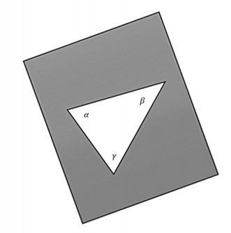
Now consider the surface of a sphere. If a triangle is constructed on the surface of the sphere by joining three points with geodesic (arc of great circles), the sum of the interior angles of the spherical triangle is greater than 180o, i.e. −
$$\alpha + \beta + \gamma > \pi$$
Such spaces are called positively curved spaces. Also, the curvature is homogeneous and isotropic. In general, the angle at the vertices of the spherical triangle follows the relation −
$$\alpha + \beta +\gamma = \pi + A/R^2$$
where A is the area of the triangle and R is the radius of the sphere. The following image depicts a positively curved space.
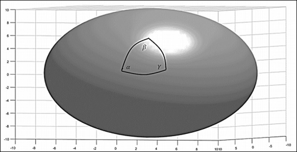
For a positive curvature, the parallel lines should meet. Consider the surface of the earth, which is a positively curved space. Take two starting points on the equator. The lines which cross the equator at right angles are known as the lines of longitude. Since these lines cross the equator at right angles, they can be referred to as parallel lines. Starting from the equator, they eventually intersect at the poles. This method was used by Carl Gauss and others to understand the topology of the earth.
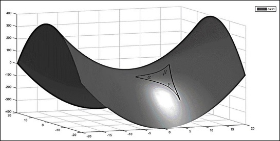
Consider a negatively curved space (a saddle shown in the following image), the sum of interior angles of the triangle is less than 180o, i.e. −
$$\alpha + \beta + \gamma < \pi$$
The angle at the vertices follows the relation −
$$\alpha + \beta + \gamma = \pi - A/R^2$$
Zero Curvature
A plane surface has zero curvature. Now for a flat space, if a plane is taken and a triangle is constructed by joining three points with geodesic (straight lines), the interior sum of angles will be −
$$\alpha + \beta + \gamma = \pi$$
The following image is a flat 2-dimensional space.
If one wants a space to be homogeneous and isotropic, only three possibilities remain: the space can be uniformly flat or it can have a uniform positive curvature or it can have a uniform negative curvature.
The curvature constant can assume any of the following three values.
$$k = \begin{cases}+1, & for \: a\: positively \: curved\: space;\\\quad 0, & for\: a \: flat \: space;\\-1, & for\: a \: negatively \: curved \: space;\end{cases}$$
Global Topology of the Universe
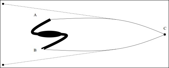
The universe has a certain topology, but locally it can have wrinkles. Depending on how the matter is distributed in the space, there are smaller variations in the curvature. Let us assume that there is a class of objects which have the same true size no matter where it is in the universe, which means they are like standard candles. They dont have the same brightness, but they have the same size.
If the object is in positively curved space and photons comes from point A (one end of the object) and B (other end of the object), the photons will propagate parallel in positively curved space through the path of geodesic and they will eventually meet. For an observer at C, it will seem that it came from two different points in different directions.
If the object is in the local universe and we measure the angular size, it is not affected by the curvature. If the same class of object is seen at a greater redshift, the angular size does not correlate with.
$$\theta = \frac{d}{r}$$
Where d is the size of the object and r is the distance to the object, i.e. if size is greater than the local size, it means the curvature is positive. The following image is a representation of the photon detected in a positively curved space.
It is to be noted that there is no real astrophysical object which is of standard size and morphology. Although a massive elliptical cD galaxies were thought to fit the standard candles, but they were also found to be evolving with time.
Finding Distances to Galaxies
In this section, we will discuss how to find the distance to a galaxy by taking into consideration the following image.
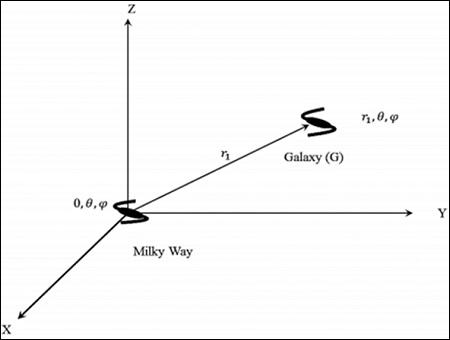
Consider the Milky Way at (r, θ,) in a cosmological rest frame. One can take = 0; (0, θ,ϕ), i.e. the centre of the universe by invoking the assumption of homogeneity.
Consider a galaxy G at (r1, θ,). The distance (proper) is the shortest radial distance travelled by a photon. From the symmetry of space time, the null geodesic from r = 0 to r = r1, has a constant direction in space. In its radial propagation, the angular co-ordinates do not change. If angular coordinates get changed, then it is not the shortest path. That is the reason why the curvature term is present in dr2.
Points to Remember
The expansion of the universe is in all the directions.
The universe can be static, expanding or contracting depending upon the scale factor evolution.
The cD-galaxies evolve with time and hence cannot be used as standard candles.
The universe has certain topology, but locally it can have wrinkles.
Hubble Parameter & Scale Factor
In this chapter, we will discuss regarding the Hubble Parameter as well as the Scale Factor.
Prerequisite − Cosmological Redshift, Cosmological Principles.
Assumption − The universe is homogenous and isotropic.
Hubbles Constant with Fractional Rate of Change of Scale Factor
In this section, we will relate the Hubbles Constant with fractional rate of Change of Scale Factor.
We can write velocity in the following manner and simplify.
$$v = \frac{\mathrm{d} r_p}{\mathrm{d} t}$$
$$= \frac{d[a(t)r_c}{dt}$$
$$v = \frac{\mathrm{d} a}{\mathrm{d} t} \ast \frac{1}{a} \ast (ar_c)$$
$$v = \frac{\mathrm{d} a}{\mathrm{d} t} \ast \frac{1}{a} \ast r_p$$
Here, v is the recessional velocity, a is the scale factor and rp is the proper distance between the galaxies.
Hubbles Empirical Formula was of the nature −
$$v = H \ast r_p$$
Thus, comparing the above two equations we obtain −
Hubbles Parameter = Fractional rate of change of the scale factor
$$H = da/dt \ast 1/a$$
Note − This is not a constant since the scale factor is a function of time. Hence it is called the Hubbles parameter and not the Hubbles constant.
Empirically we write −
$$H = V/D$$
Thus, from this equation, we can infer that since D is increasing and V is a constant, then H reduces with the time and expansion of the universe.
Friedmann Equation in Conjunction with the Robertson-Walker Model
In this section, we will understand how the Friedmann Equation is used in conjunction with the Robertson-Walker model. To understand this, let us take the following image which has a test mass at distance rp from body of mass M as an example.
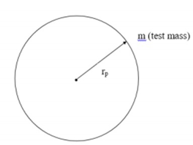
Taking into consideration the above image, we can express force as −
$$F = G \ast M \ast \frac{m}{r^2_p}$$
Here, G is the universal gravitational constant and ρ is the matter density inside the observable universe.
Now, assuming uniform mass density within the sphere we can write −
$$M = \frac{4}{3} \ast \pi \ast r_p^3 \ast \rho$$
Using these back in our force equation we get −
$$F = \frac{4}{3} \ast \pi \ast G \ast r_p \ast \rho \ast m$$
Thus, we can write the potential energy and kinetic energy of the mass m as −
$$V = -\frac{4}{3} \ast \pi \ast G \ast r^2_p \ast m \ast \rho$$
$$K.E = \frac{1}{2} \ast m \ast \frac{\mathrm{d} r_p^2}{\mathrm{d} t}$$
Using the Virial Theorem −
$$U = K.E + V$$
$$U = \frac{1}{2} \ast m \ast \left ( \frac{\mathrm{d} r_p}{\mathrm{d} t} \right )^2 - \frac{4}{3} \ast \pi \ast G \ast r_p^2 \ast m \ast \rho$$
But here, $r_p = ar_c$. So, we get −
$$U = \frac{1}{2} \ast m \ast \left ( \frac{\mathrm{d} a}{\mathrm{d} t} \right )^2 r_c^2 - \frac{4}{3} \ast \pi \ast G \ast r_p^2 \ast m \ast \rho$$
On further simplification, we obtain the Friedmann equation,
$$\left ( \frac{\dot{a}}{a} \right )^2 = \frac{8\pi}{3} \ast G \ast \rho + \frac{2U}{m} \ast r_c^2 \ast a^2$$
Here U is a constant. We also note that the universe we live in at present is dominated by matter, while the radiation energy density is very low.
Points to Remember
The Hubble parameter reduces with time and expansion of the universe.
The universe we live in at present is dominated by matter and radiation energy density is very low.
Friedmann Equation & World Models
In this chapter, we will understand what the Friedmann Equation is and study in detail regarding the World Models for different curvature constants.
Friedmann Equation
This equation tells us about the expansion of space in homogeneous and isotropic models of the universe.
$$\left ( \frac{\dot{a}}{a} \right )^2 = \frac{8\pi G}{3}\rho + \frac{2U}{mr_c^2a^2}$$
This was modified in context of General Relativity (GR) and Robertson-Walker Metric as follows.
Using GR equations −
$$\frac{2U}{mr_c^2} = -kc^2$$
Where k is the curvature constant. Therefore,
$$\left ( \frac{\dot{a}}{a} \right )^2 = \frac{8 \pi G}{3}\rho - \frac{kc^2}{a^2}$$
Also, $\rho$ is replaced by energy density which includes matter, radiation and any other form of energy. But for representational purposes, it is written as $\rho$.
World Models for Different Curvature Constants
Let us now look at the various possibilities depending on the curvature constant values.
Case 1: k=1, or Closed Universe
For an expanding universe, $da/dt > 0$. As expansion continues, the first term on the RHS of the above equation goes as $a^{-3}$, whereas the second term goes as $a^{-2}$. When the two terms become equal the universe halts expansion. Then −
$$\frac{8 \pi G}{3}\rho = \frac{kc^2}{a^2}$$
Here, k=1, therefore,
$$a = \left [ \frac{3c^2}{8 \pi G\rho} \right ]^{\frac{1}{2}}$$
Such a universe is finite and has finite volume. This is called a Closed Universe.
Case 2: k=-1, or Open Universe
If k < 0, the expansion would never halt. After some point, the first term on the RHS can be neglected in comparison with the second term.
Here, k = -1. Therefore, $da/dt ∼ c$.
In this case, the universe is coasting. Such a universe has infinite space and time. This is called an Open Universe.
Case 3: k=0, or Flat Universe
In this case, the universe is expanding at a diminishing rate. Here, k = 0. Therefore,
$$\left ( \frac{\dot{a}}{a} \right )^2 = \frac{8\pi G}{3}\rho$$
Such a universe has infinite space and time. This is called a Flat Universe.
Points to Remember
The Friedmann equation tells us about the expansion of space in homogeneous and isotropic models of the universe.
Depending on different curvature constant values, we can have a Closed, Open or Flat Universe.
Cosmology - Fluid Equation
In this chapter, we will discuss Fluid Equation and how it tells us regarding the density of universe that changes with time.
Estimating ρc and ρ in the Present Universe
For the present universe −
$$\rho_c \simeq 10^{11}M_\odot M_{pc}^{-3} \simeq 10\: hydrogen \: atoms \: m^{-3}$$
There is a whole range of critical density in our outer space. Like, for intergalactic medium $\rho_c$ is 1 hydrogen atom $m^{-3}$, whereas for molecular clouds it is $10^6$ hydrogen atoms $m^{3}$.
We must measure $\rho_c$ considering proper samples of space. Within our galaxy, the value of $\rho_c$ is very high, but our galaxy is not a representative of the whole universe. So, we should go out to space where cosmological principle holds, i.e., distances ≈ 300 Mpc. Looking at 300 Mpc means looking 1 billion years back, but it is still the present universe.
Surveys like SDSS are conducted to determine the actual matter density. They take a 55005 Mpc3 volume, count the number of galaxies and add all the light coming from these galaxies. Under an assumption that 1 L ≡ 1 M, i.e. 1 solar Luminosity ≡ 1 solar Mass.
We do a light to mass conversion and then we try to estimate the number of baryons based on the visible matter particles present in that volume.
For example,
$$1000L_\odot ≡ 1000M_\odot / m_p$$
Where, mp= mass of proton.
Then we get roughly the baryon number density $\Omega b ∼= 0.025$. This implies $\rho b = 0.25%$ of $\rho_c$. Different surveys have yielded a slightly different value. So, in the local universe, number density of visible matter is much less than critical density, meaning we are living in an open universe.
Mass with a factor of 10 is not included in these surveys because these surveys account for electromagnetic radiation but not dark matter. Giving, $\Omega_m = 0.3 0.4$. Still concludes that we are living in an open universe.
Dark matter interacts with gravity. A lot of dark matter can halt the expansion. We havent yet formalized how $\rho$ changes with time, for which we need another set of equations.
Thermodynamics states that −
$$dQ = dU + dW$$
For a system growing in terms of size, $dW = P dV$. Expansion of universe is modelled as adiabatic i.e. $dQ = 0$. So, volume change should happen from change in internal energy dU.
Let us take a certain volume of universe of unit comoving radius i.e. $r_c = 1$. If $\rho$ is the density of material within this volume of space, then,
$$M = \frac{4}{3} \pi a^3r_c^3 \rho$$
$$U = \frac{4}{3}\pi a^3\rho c^2$$
Where, U is the Energy density. Let us find out the change in internal energy with time as the universe is expanding.
$$\frac{\mathrm{d} U}{\mathrm{d} t} = 4 \pi a^2 \rho c^2 \frac{\mathrm{d} a}{\mathrm{d} t} + \frac{4}{3}\pi a^3 c^2\frac{\mathrm{d} \rho}{\mathrm{d} t}$$
Similarly, change in volume with time is given by,
$$\frac{\mathrm{d} V}{\mathrm{d} t} = 4\pi a^2 \frac{\mathrm{d} a}{\mathrm{d} t}$$
Substituting $dU = P dV$. We get,
$$4\pi a^2(c^2 \rho +P)\dot{a}+\frac{4}{3}\pi a^3c^2\dot{\rho} = 0$$
$$\dot{\rho}+3\frac{\dot{a}}{a}\left ( \rho + \frac{P}{c^2} \right ) = 0$$
This is called the Fluid Equation. It tells us how the density of universe changes with time.
Pressure drops as the universe expands. At every instant pressure is changing, but there is no pressure difference between two points in the volume considered, so, the pressure gradient is zero. Only relativistic materials impart pressure, matter is pressure-less.
Friedmann Equation along with Fluid Equation models the universe.
Points to Remember
Dark matter interacts with gravity. A lot of dark matter can halt the expansion.
Fluid Equation tells us how the density of universe changes with time.
Friedmann Equation along with Fluid Equation models the universe.
Only relativistic materials impart pressure, matter is pressure-less.
Cosmology - Matter Dominated Universe
In this chapter, we will discuss the Solutions to Friedmann Equations relating to the Matter Dominated Universe. In cosmology, because we are seeing everything in a large scale, the solar systems, galaxies, everything happens to be like dust particles (thats what we see it with our eyes), we can call it dusty universe or matter only universe.
In the Fluid Equation,
$$\dot{\rho} = -3\left ( \frac{\dot{a}}{a} \right )\rho -3\left ( \frac{\dot{a}}{a} \right )\left ( \frac{P}{c^2} \right )$$
We can see there is a pressure term. For a dusty universe, P = 0, because the energy density of the matter will be greater than radiation pressure, and matter is not moving with relativistic speed.
So, the Fluid Equation will become,
$$\dot{\rho} = -3\left ( \frac{\dot{a}}{a} \right )\rho$$
$$\Rightarrow \dot{\rho}a + 3\dot{a}\rho = 0$$
$$\Rightarrow \frac{1}{a^3}\frac{\mathrm{d}}{\mathrm{d} t}(a^3 \rho) = 0$$
$$\Rightarrow \rho a^3 =\: constant$$
$$\Rightarrow \rho \propto \frac{1}{a^3}$$
There is no counter intuition in this equation because density should scale as $a^{-3}$ because Volume is increasing as $a^3$.
From the last relation, we can say that,
$$\frac{\rho (t)}{\rho_0} = \left [ \frac{a_0}{a(t)} \right ]^3$$
For the present universe, a, which is equal to a0 should be 1. So,
$$\rho(t) = \frac{\rho_0}{a^3}$$
In a matter dominated flat universe, k = 0. So, Friedmann equation will become,
$$\left ( \frac{\dot{a}}{a} \right )^2 = \frac{8 \pi G\rho}{3}$$
$$\dot{a}^2 = \frac{8\pi G \rho a^2}{3}$$
By solving this equation, we will get,
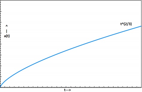
$$a \propto t^{2/3}$$
$$\frac{a(t)}{a_0} = \left ( \frac{t}{t_0} \right )^{2/3}$$
$$a(t) = \left( \frac{t}{t_0} \right )^{2/3}$$
This means that the universe will keep on increasing with a diminishing rate. The following image show the expansion of a Dusty Universe.
How ρ Changes with Time?
Take a look at the following equation −
$$\frac{\rho(t)}{\rho_0} = \left ( \frac{t_0}{t} \right )^2$$
We know that the scale factor changes with time as $t^{2/3}$. So,
$$a(t) = \left ( \frac{t}{t_0} \right )^{2/3}$$
Differentiating it, we will get,
$$\frac{(da)}{dt} = \dot{a} = \frac{2}{3} \left ( \frac{t^{-1/3}}{t_0} \right )$$
We know that the Hubble Constant is,
$$H(t) = \frac{\dot{a}}{a} = \frac{2}{3t}$$
This is the equation for Einstein-de sitter Universe. If we want to calculate the present age of the universe then,
$$t_0 = t_{age} = \frac{2}{3H_0}$$
After putting the value of $H_0$ for the present universe, we will get the value of the age of the universe as 9 Gyrs. There are many Globular Cluster in our own milky way galaxy which have ages more than that.
That was all about the dusty universe. Now, if you assume that the universe is dominated by radiation and not by matter, then the radiation energy density goes as $a^{-4}$ rather than $a^{-3}$. We will see more of it in the next chapter.
Points to Remember
In cosmology, everything happens to be like dust particles, hence, we call it dusty universe or matter only universe.
If we assume that the universe is dominated by radiation and not by matter, then the radiation energy density goes as $a^{-4}$ rather than $a^{-3}$.
Cosmology - Radiation Dominated Universe
In this chapter, we will discuss the Solutions to Friedmann Equations relating to the Radiation Dominated Universe. In the beginning, we compare the energy density of matter to that of radiation. This will enable us to see if our universe is matter dominated or radiation dominated.
Energy Density of Radiation
Radiation prevalent in the present universe can be attributed very little to the stellar sources, but it is mainly due to the remnant CMB (Cosmic Microwave Background).
The energy density of the radiation, $\epsilon_{\gamma,0}$, can be expressed as follows −
$$\epsilon_{\gamma,0} = aT_0^4$$
Here, a is the radiation constant which has the expression $(8\pi^5k_B^4)/(15h^3c^2)$ equal to a = 7.5657 1015erg\: cm3 K4. The Temperature, T0, we consider here, corresponds to that of the black body corresponding to the CMB.
Substituting the results, we have,
$$\epsilon_{\gamma,0} = aT_0^4 = 4 \times 10^{-13}erg\: cm^{-3}$$
Energy Density of Matter
In the following calculations, we have the assumption of working with a flat universe and K = 0. We consider the energy density of matter as $\epsilon = \rho c^2$. We consider the following −
$$\rho_{m,0}c^2 = 0.3\rho_{c,0}c^2 = 0.3 \times \frac{3H_0^2}{8\pi G} \times c^2$$
$$\rho_{m,0}c^2 \simeq 2 \times 10^{-8} erg \:cm^{-3}$$
$$\rho_{b,0}c^2 = 0.03\rho_{c,0}c^2 = 0.03 \times \frac{3H_0^2}{8\pi G} \times c^2$$
$$\rho_{b,0}c^2 \simeq 2 \times 10^{-9} erg\: cm^{-3}$$
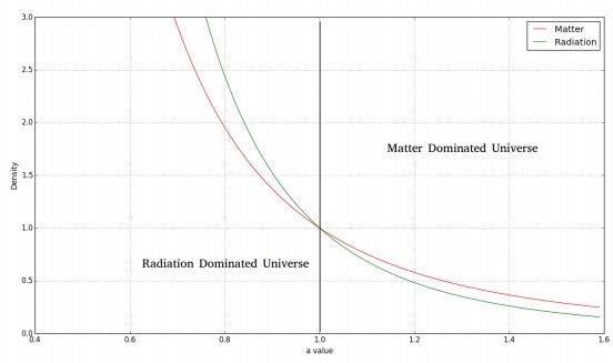
Thus, from the above calculation, we see that we live in a matter-dominated universe. This can be supported by the fact that the CMB is very cold. As we look back in time, we would have the CMB temperature getting hotter, and will be able to conclude that there might have been an epoch where the universe was dominated by radiation.
Variation of Density and Scale Factor
The fluid equation shows us that −
$$\dot{\rho} + 3\frac{\dot{a}}{a}\left ( \rho + \frac{P}{c^2} \right ) = 0$$
If we consider a dusty universe, we would have P = 0. Setting aside the previous results, we consider the universe as dominated by radiation.
$$\dot{\rho}_{rad} + 3 \frac{\dot{a}}{a}\left ( \rho_{rad} + \frac{P}{c^2} \right ) = 0$$
Using the pressure relation of $P_{rad} = \rho c^{2/3}$ we have −
$$\dot{\rho}_{rad} + 3 \frac{\dot{a}}{a}\left ( \rho_{rad} + \frac{\rho_{rad}}{3} \right ) = 0$$
$$\dot{\rho}_{rad} + 4\frac{\dot{a}}{a}(\rho_{rad}) = 0$$
On further simplification, we have,
$$\frac{1}{a^4}\frac{\mathrm{d}}{\mathrm{d} t}(\rho_{rad}a^4) = 0$$
$$\rho_{rad}a^4 =\: constant$$
$$\rho_{rad} \propto \frac{1}{a^4}$$
The above result shows an inverse 4th power variation of a with $\rho$.
This can be physically interpreted as $a^{-3}$ coming in from the variation in volume as it increases. The remaining $a^{-1}$ can be treated as the energy lost by the photon due to the expansion of space in the universe (Cosmological redshift 1 + z = a-1).
The following image shows the variation of matter and radiation density with time.
For a flat, radiation dominated universe, we would have the Friedmann equation as follows −
$$\left ( \frac{\dot{a}}{a} \right )^2 = \frac{8\pi G\rho}{3}$$
$$\left ( \frac{\dot{a}}{a} \right)^2 = \frac{8\pi G}{3}\frac{\rho_0}{a^4}$$
On simplification and applying the solution to the differential equation, we have −
$$(\dot{a})^2 = \frac{8\pi G\rho_0}{3a^2}$$
$$\Rightarrow a(t) \propto t^{\frac{1}{2}}$$
Thus, we have −
$$a(t) = a_0 \left ( \frac{t}{t_0} \right )^{\frac{1}{2}}$$
From the above equation, we see that the rate of increase of scale factor is smaller than that of the dusty universe.
Points to Remember
Radiation prevalent in the present universe can be attributed very little to the stellar sources.
For a dusty universe, pressure is zero.
CMB is very cold.
Cosmology - Dark Energy
The area of Dark Energy is a very grey area in astronomy because it is a free parameter in all equations, but there is no clear idea what exactly this is.
We will start with the Friedmanns equations,
$$\left ( \frac{\dot{a}}{a} \right)^2 = \frac{8\pi G}{3}\rho - \frac{k \ast c^2}{a^2}$$
Most of the elementary books on cosmology, they all start with describing the dark energy from this episode that before Hubbles observation, the universe is closed and static.
Now, for the universe to be static in the right side, both the terms should match and they should be zero, but if the first term is greater than the second term, then the universe will not be static, so Einstein dropped the free parameter ∧ into the field equation to make the universe static, so he argued that no matter what the first term is compared to the second term, you can always get a static universe if there is one more component in the equation, which can compensate the dis-match between these two terms.
$$\left ( \frac{\dot{a}}{a} \right )^2 = \frac{8\pi G}{3}\rho - \frac{k \ast c^2}{a^2} + \frac{\wedge}{3}$$
$$\left ( \frac{\ddot{a}}{a} \right ) = -\frac{4 \pi G}{3}\left ( \rho + \frac{3P}{c^2} \right ) + \frac{\wedge}{3}$$
Where $P = \rho \ast c^2/3$ and $\wedge = \rho \ast c^2$ is the Cosmological Parameter. (Negative sign is only because of attraction)
In the above equation (acceleration equation) −
$3P/c^2$ is the negative pressure due to radiation,
$-4\pi G/3$ is the attraction due to gravity, and
$\wedge/3$ makes a positive contribution.
The third term acts as a repulsive force because another part of the equation is attractive.
The physical significance of the equation is that a = 0 because there was not any evidence which shows that the universe is expanding. What if these two terms are not matching with each other, so it is better to add a component and depending on the offset we can always change the value of the free parameter.
That time there was no physical explanation about this cosmological parameters, which is why when the explanation of the expanding universe was discovered in 1920s, where Einstein immediately had to throw this constant out.
The explanation of this cosmological constant is still in use because it explains a different version of the universe, but the definition of this cosmological constant, the way of interpretation kept changing with time.
Now the concept of this cosmological constant has been brought back to cosmology for many reasons. One of the reason is that, we have observations for energy density of different components of the universe (baryonic, dark matter, radiation), so we know that what this parameter is. Independent observations using cosmic microwave background shows that k=0.
$$CMB, k=0\: \rho = \rho_c = \frac{3H_0^2}{8\pi G} \approx 10 \: Hydrogen \: atoms.m^{-3}$$
For k to be 0, $\rho$ should be equal to $\rho_c$, but everything we know if we add it up that does not give 0, which means that there is some other component that shows that it is much less than $\rho_c$.
$$\rho = \rho_b + \rho_{DM} + \rho_{rad} << \rho_c$$
One more evidence of dark energy comes from the Type 1 Supernova Observation which occurs when white dwarf accretes the matter and exceeds the Chandrashekhar limit, which is a very precise limit (≈ 1.4M). Now every time when Type 1 Supernova Explosion occurs, we have the same mass which means that the total binding energy of the system is same and the amount of light energy we can see is the same.
Of course, the supernova light increases and then faints, but if you measure the peak brightness it is always going to be the same which makes it a standard candidate. So, with a Type 1 Supernova we used to measure the cosmological component of the universe and astronomers found that the supernova with high red shift is 30% 40% fainter than the low red shift supernova and it can be explained if there is any non-zero ∧ term.
In cosmological models DE (Dark Energy) is treated as a fluid, which means that we can write the equation of state for it. The equation of state is the equation which connects the variables like Pressure, Density, Temperature, and Volume of two different states of the matter.
Dimensionally we see,
$$\frac{8 \pi G}{3}\rho = \frac{\wedge}{3}$$
$$\rho_\wedge = \frac{\wedge}{8\pi G}$$
Energy density of DE,
$$\epsilon_\wedge = \rho_\wedge \ast c^2 = \frac{\wedge c^2}{8 \pi G}$$
Dark energy density parameter,
$$\Omega_\wedge = \frac{\rho_\wedge}{\rho_c}$$
$\Omega_\wedge$ is the density of dark energy in terms of critical density.
$$\rho = \rho_b + \rho_{DM} +\rho_\wedge$$
There are a number of theories about dark energy, which is repelling the universe and causing the universe to expand. One hypothesis is that this dark energy could be a vacuum energy density. Suppose the space itself is processing some energy and when you count the amount of baryonic matter, dark matter and the radiation within the unit volume of space, you are also counting the amount of energy which is associated with the space, but it is not clear that the dark energy is really a vacuum energy density.
We know that the relationship between density and scale factor for dark matter and radiation are,
$$\rho_m \propto \frac{1}{a^3}$$
$$\rho_m \propto \frac{1}{a^4}$$
We have the density v/s scale factor plot. In the same plot, we can see that $\rho_\wedge$ is a constant with the expansion of the universe which does not depend on the scale factor.
The following image shows the relationship between density and the scale factor.
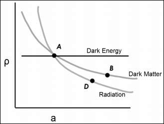
ρ v/s a (scale factor which is related to time) in the same graph, the dark energy is modelled as a constant. So, whatever dark energy we measure in the present universe, it is a constant.
Points to Remember
Independent observations using cosmic microwave background shows that k=0.
$\rho_\wedge$ is a constant with the expansion of the universe which does not depend on the scale factor.
Gravity is also changing with time which is called modified Newtonian dynamics.
Cosmology - Spiral Galaxy Rotation Curves
In this chapter, we will discuss regarding Spiral Galaxy Rotation Curves and evidence for Dark Matter.
Dark Matter and Observational Fact about Dark Matter
The Early Evidence of Dark Matter was the study of the Kinematics of Spiral Galaxy.
The Sun is offset 30,000 lightyears from the centre of our Galaxy. The galactic centric velocity is 220 km/s.
Why is the velocity 220 km/s not 100 km/s or 500 km/s? What governs the circular motion of object?
Mass enclosed within the radius helps to detect the velocity in the Universe.
Rotation of Milky Way or Spiral Galaxy Differential Rotation
Angular Velocity varies with the distance from the centre.
Orbital time-period depends on the distance from the centre.
Material closer to Galactic centre has a shorter time-period and material far away from the Galactic Centre has a larger time period.
Rotation Curve
Predict the velocity change with the Galactic centric radius. The curve which gives the velocity changes with the orbital radius.
When we see things move, we think that it is gravity which influences the rotation.
Mass distribution varies with the radius. Matter density will predict the rotation curve. The rotation curve based on the matter density, which varies with radius.
Surface Brightness
We choose the patch and see how much of light is coming out.
Amount of the light coming from the patch is called as the Surface Brightness.
Its unit is mag/arcsec2.
If we find the surface brightness varies with the radius, we can find the luminous matter varies with radius.
$$\mu(r) \propto exp \left( \frac{-r}{h_R} \right )$$
$h_R$ is scale length. $\mu(r) = \mu_o \ast exp \left( \frac{-r}{h_R} \right )$
$h_R$ is nearly 3 kpc for the Milky way.
Spiral Galaxies
For the Astronomers to understand the rotational curve, they split the Galaxies into two components, which are −
- Disk
- Bulge
The following image shows a Central spherical bulge + Circular disk. Stellar and gas distribution is different in the bulge and the disk.
Kinematics of Spiral Galaxies
-
The Circular velocity of any object For the bulge is (r < Rb).
$$V^2(r) = G \ast \frac{M(r)}{r}$$
$$M(r) = \frac{4\pi r^3}{3} \ast \rho_b$$
-
For the disk (Rb < r < Rd)
$$V^2(r) = G \ast \frac{M(r)}{r}$$
Bulge has a roughly constant density of stars.
Density within the Bulge is constant (not changing with the distance within the bulge).
In a disk, the stellar density declines with the radius. The radius increases then the luminous matter decrease.
In Bulk $V(r) \propto r$
In Disc $V(r) \propto 1/\sqrt{r}$
Rotational Curve of Spiral Galaxies
Through the Spectroscopy (nearby galaxies spatially resolved the galaxy), we produce the rotation curve.
As mentioned above, we see that the rotation curve is flat at the outer regions, i.e. the things are moving fast in the outer regions, which is generally not expected to be in this form.
The orbital speed increases with the increase in the radius of the inner region, but it flattens in the outer region.
Dark Matter
The Dark Matter is said to be the Non-Luminous Component of the Universe. Let us understand about dark matter through the following pointers.
The flat rotation curves are counter to what we see for the distribution of stars and gas in the spiral galaxies.
The surface luminosity of the disk falls off exponentially with radius, implying that the mass of luminous matter, mostly stars, is concentrated around the galactic center.
The flattening of the rotation curve suggests that the total mass of the galaxy within some radius r is increasing always with increase in r.
This can only be explained if there is a large amount of invisible gravitating mass in these galaxies which is not giving out electromagnetic radiation.
The rotation curve measurements of spiral galaxies is one of the most compelling set of evidences for dark matter.
Evidence of Dark Matter
Missing Mass 10 times the luminous mass.
Most of this dark matter must be in the halo of the galaxy: Large amounts of dark matter in the disk can disturb the long-term stability of the disk against tidal forces.
Some small fraction of the dark matter in the disk can be baryonic dim stars (brown dwarfs, black dwarfs), and compact stellar remnants (neutron stars, black holes). But such baryonic dark matter cannot explain the full scale of missing mass in galaxies.
Density Profile of Dark Matter $M(r) \propto r$ and $\rho(r) \propto r^{2}$.
The rotation curve data for spiral galaxies are consistent with the dark matter distributed in their halo.
This dark halo constitutes much of the galaxys total mass.
All baryonic matter (stars, star clusters, ISM, etc.) are held together by the gravitational potential of this dark matter halo.
Conclusion
Dark matter has only been detected through their gravitational interaction with an ordinary matter. No interaction with light (no electromagnetic force) has yet been observed.
Neutrinos − Charge less, weakly interacting, but mass is too less (< 0.23 eV). DM particles should have E > 10 eV or so to explain structure formation.
Weakly Interacting Massive Particles (WIMPS) can be the source of Dark Matter.
Points to Remember
Material closer to Galactic centre has a shorter time-period.
Bulge has a roughly constant density of stars.
Surface luminosity of the disk falls off exponentially with radius.
Large amounts of dark matter in the disk can disturb the long-term stability of the disk against tidal forces.
Velocity Dispersion Measurements of Galaxies
First direct evidence of dark matter came from Frids Ricky. He did some observations which revealed dark matter for the first time. His observations considered the overall motion within the galaxy cluster.
Extended objects are galaxy clusters and they are considered bound structures. These galaxies are moving with respect to cluster center but do not fly off. We look at the overall motion of the galaxy.
Assumption: Velocities are Represent of Underlying Potential
Every galaxy will have its own proper motion within the cluster and Hubble Flow Component. The smaller galaxies are smaller, most of the light comes from M31 and MW, there are several dwarf galaxies. For our crude analysis, we can only use M31 and MW and evaluate dynamic mass of the local group.
There is a relative velocity between us and M31. It is crude, but it is true. The story begins long back when M31 and MW were close to each other, because they were members of a cluster they were moving away from each other. After some time they reach the maximum separation, then come closer to each other.
Let us say that the maximum separation that can ever reach is $r_{max}$. Now they have a separation called r. Let M be the combined mass of MW and M31. We do not know when $r_{max}$ is reached.
$$\frac{GM}{r_{max}} = \:Potential \: at \:r_{max}$$
When these galaxies were coming close to each other at some instant r, then the energy of the system will be −
$$\frac{1}{2}\sigma^2 = \frac{GM}{r} = \frac{GM}{r_{max}}$$
σ is relative velocity of both the galaxies. M is reduced mass only, but the test mass is 1. σ is velocity of any object at distance r from the centre of the cluster. We believe that this cluster is in dynamic equation because virial theorem holds. So, galaxies cannot come with different velocity.
How much time would these galaxies take to reach the maximum distance?
To understand this, let us consider the following equation.
$$\frac{1}{2}\left ( \frac{dr}{dt} \right )^2 = \frac{GM}{r} - \frac{GM}{r_{max}}$$
$$t_{max} = \int_{0}^{r_{max}} dt = \int_{0}^{r_{max}} \frac{dr}{\sqrt{2GM}}\left ( \frac{1}{r} - \frac{1}{r_{max}} \right )^2$$
$$t_{max} = \frac{\pi r_{max}^{\frac{3}{2}}}{2\sqrt{2GM}}$$
Where, M = dynamical mass of local group. The Total time from the start till the end of collision is $2t_{max}$. Therefore,
$$2t_{max} = t_0 + \frac{D}{\sigma}$$
And $t_0$ is the present age of universe.
If actual $t_{max} < RHS$, then we have a lower limit for the time. $D/\sigma$ is the time when they will collide again. Here, we have assumed σ to be constant.
$$t_{max} = \frac{t_0}{2} + \frac{D}{2\sigma}$$
$$r_{max} = t_{max} \times \sigma = 770K_{pc}$$
Here, σ = relative velocity between MW and M31.
$$M_{dynamic} = 3 \times 10^{12}M_0$$
$$M_{MW}^{lum} = 3 \times 10^{10}M_0$$
$$M_{M31}^{lum} = 3 \times 10^{10}M_0$$
But practically, dynamic mass is found out considering every galaxy within the cluster. The missing mass is the dark matter and Frids Ricky noticed that the galaxies in the coma cluster are moving too fast. He predicted the existence of neutron stars the year after neutron stars were discovered and used Palomar telescope to find the supernova.
Points to Remember
First direct evidence of dark matter came from Frids Ricky.
Extended objects are galaxy clusters and they are considered bound structures.
Dynamic mass is found out considering every galaxy within the cluster.
Cosmology - Hubble & Density Parameter
In this chapter, we will discuss regarding the Density and Hubble parameters.
Hubble Parameter
The Hubble parameter is defined as follows −
$$H(t) \equiv \frac{da/dt}{a}$$
which measures how rapidly the scale factor changes. More generally, the evolution of the scale factor is determined by the Friedmann Equation.
$$H^2(t) \equiv \left ( \frac{\dot{a}}{a} \right )^2 = \frac{8\pi G}{3}\rho - \frac{kc^2}{a^2} + \frac{\wedge}{3}$$
where, ∧ is a cosmological constant.
For a flat universe, k = 0, hence the Friedmann Equation becomes −
$$\left ( \frac{\dot{a}}{a} \right )^2 = \frac{8\pi G}{3}\rho + \frac{\wedge}{3}$$
For a matter dominated universe, the density varies as −
$$\frac{\rho_m}{\rho_{m,0}} = \left ( \frac{a_0}{a} \right )^3 \Rightarrow \rho_m = \rho_{m,0}a^{-3}$$
and, for a radiation dominated universe the density varies as −
$$\frac{\rho_{rad}}{\rho_{rad,0}} = \left ( \frac{a_0}{a} \right )^4 \Rightarrow \rho_{rad} = \rho_{rad,0}a^{-4}$$
Presently, we are living in a matter dominated universe. Hence, considering $\rho \rho_m$, we get −
$$\left ( \frac{\dot{a}}{a} \right )^2 = \frac{8\pi G}{3}\rho_{m,0}a^{-3} + \frac{\wedge}{3}$$
The cosmological constant and dark energy density are related as follows −
$$\rho_\wedge = \frac{\wedge}{8 \pi G} \Rightarrow \wedge = 8\pi G\rho_\wedge$$
From this, we get −
$$\left ( \frac{\dot{a}}{a} \right )^2 = \frac{8\pi G}{3}\rho_{m,0}a^{-3} + \frac{8 \pi G}{3} \rho_\wedge$$
Also, the critical density and Hubbles constant are related as follows −
$$\rho_{c,0} = \frac{3H_0^2}{8 \pi G} \Rightarrow \frac{8\pi G}{3} = \frac{H_0^2}{\rho_{c,0}}$$
From this, we get −
$$\left ( \frac{\dot{a}}{a} \right )^2 = \frac{H_0^2}{\rho_{c,0}}\rho_{m,0}a^{-3} + \frac{H_0^2}{\rho_{c,0}}\rho_\wedge$$
$$\left ( \frac{\dot{a}}{a} \right )^2 = H_0^2\Omega_{m,0}a^{-3} + H_0^2\Omega_{\wedge,0}$$
$$(\dot{a})^2 = H_0^2\Omega_{m,0}a^{-1} + H_0^2\Omega_{\wedge,0}a^2$$
$$\left ( \frac{\dot{a}}{H_0} \right )^2 = \Omega_{m,0}\frac{1}{a} + \Omega_{\wedge,0}a^2$$
$$\left ( \frac{\dot{a}}{H_0} \right )^2 = \Omega_{m,0}(1+z) + \Omega_{\wedge,0}\frac{1}{(1+z)^2}$$
$$\left ( \frac{\dot{a}}{H_0} \right)^2 (1+z)^2 = \Omega_{m,0}(1+z)^3 + \Omega_{\wedge,0}$$
$$\left ( \frac{\dot{a}}{H_0} \right)^2 \frac{1}{a^2} = \Omega_{m,0}(1 + z)^3 + \Omega_{\wedge,0}$$
$$\left ( \frac{H(z)}{H_0} \right )^2 = \Omega_{m,0}(1+z)^3 + \Omega_{\wedge,0}$$
Here, $H(z)$ is the red shift dependent Hubble parameter. This can be modified to include the radiation density parameter $\Omega_{rad}$ and the curvature density parameter $\Omega_k$. The modified equation is −
$$\left ( \frac{H(z)}{H_0} \right )^2 = \Omega_{m,0}(1+z)^3 + \Omega_{rad,0}(1+z)^4+\Omega_{k,0}(1+z)^2+\Omega_{\wedge,0}$$
$$Or, \: \left ( \frac{H(z)}{H_0} \right)^2 = E(z)$$
$$Or, \: H(z) = H_0E(z)^{\frac{1}{2}}$$
where,
$$E(z) \equiv \Omega_{m,0}(1 + z)^3 + \Omega_{rad,0}(1+z)^4 + \Omega_{k,0}(1+z)^2+\Omega_{\wedge,0}$$
This shows that the Hubble parameter varies with time.
For the Einstein-de Sitter Universe, $\Omega_m = 1, \Omega_\wedge = 0, k = 0$.
Putting these values in, we get −
$$H(z) = H_0(1+z)^{\frac{3}{2}}$$
which shows the time evolution of the Hubble parameter for the Einstein-de Sitter universe.
Density Parameter
The density parameter, $\Omega$, is defined as the ratio of the actual (or observed) density to the critical density $\rho_c$. For any quantity $x$ the corresponding density parameter, $\Omega_x$ can be expressed mathematically as −
$$\Omega_x = \frac{\rho_x}{\rho_c}$$
For different quantities under consideration, we can define the following density parameters.
| S.No. | Quantity | Density Parameter |
|---|---|---|
| 1 | Baryons | $\Omega_b = \frac{\rho_b}{\rho_c}$ |
| 2 | Matter(Baryonic + Dark) | $\Omega_m = \frac{\rho_m}{\rho_c}$ |
| 3 | Dark Energy | $\Omega_\wedge = \frac{\rho_\wedge}{\rho_c}$ |
| 4 | Radiation | $\Omega_{rad} = \frac{\rho_{rad}}{\rho_c}$ |
Where the symbols have their usual meanings.
Points to Remember
The evolution of the scale factor is determined by the Friedmann Equation.
H(z) is the red shift dependent Hubble parameter.
The Hubble Parameter varies with time.
The Density Parameter is defined as the ratio of the actual (or observed) density to the critical density.
Cosmology - Age of Universe
As discussed in the earlier chapters, the time evolution of the Hubble parameter is given by −
$$H(z) = H_0E(z)^{\frac{1}{2}}$$
Where z is the red shift and E(Z) is −
$$E(z) \equiv \Omega_{m,0}(1+z)^3 + \Omega(1+z)^4 +\Omega_{k,0}(1+z)^2 + \Omega^{\wedge,0}$$
If the expansion of the universe is constant, then the true age of the universe is given as follows −
$$t_H = \frac{1}{H_0}$$
If it is the matter dominated universe, i.e., Einstein Desitter universe, then the true age of universe is given by −
$$t_H = \frac{2}{3H_0}$$
Scale and Redshift is defined by −
$$a=\frac{a_0}{1+z}$$
Age of the universe in terms of the cosmological parameter is derived as follows.
The Hubble Parameter is given by −
$$H = \frac{\frac{da}{dt}}{a}$$
Differentiating, we get −
$$da = \frac{-dz}{(1+z)^2}$$
Where a0 = 1 (present value of the scale factor)
$$\frac{\mathrm{d} a}{\mathrm{d} t} = \frac{-1}{(1+z)^2}$$
$$\frac{\mathrm{d} a}{\mathrm{d} t} = \frac{\mathrm{d} a}{\mathrm{d} t}\frac{\mathrm{d} z}{\mathrm{d} t}$$
$$H = \frac{\dot{a}}{a} = \frac{\mathrm{d} a}{\mathrm{d} t}\frac{\mathrm{d} z}{\mathrm{d} t} \frac{1+z}{1}$$
$$\frac{\dot{a}}{a} = \frac{-1}{1+z}\frac{\mathrm{d} z}{\mathrm{d} t}\frac{1}{1}$$
$$H(z) = H_0E(z)^{\frac{1}{2}}$$
$$dt = \frac{-dz}{H_0E(z)^{\frac{1}{2}}(1+z)}$$
If we want to find the age of the universe at any given redshift z then −
$$t(z) = \frac{1}{H_0}\int_{\infty}^{z_1} \frac{-1}{E(z)^{\frac{1}{2}}(1+z)}dz$$
Where k is the curvature density parameter and −
$$E(z) \equiv \Omega_{m,0}(1+z)^3 + \Omega_{rad,0}(1+z)^4 + \Omega_{k,0}(1+z)^2 + \Omega_{\wedge,0}$$
To calculate the present age of the universe, take z1 = 0.
$$t(z=0) = t_{age} = t_0 = \frac{1}{H_0}\int_{\infty}^{z_1} \frac{-1}{E(z)^{\frac{1}{2}}(1+z)}dz$$
For the Einstein Desitter Model, i.e, $\Omega_m = 1$, $\Omega_{rad} = 0$, $\Omega_k = 0$, $\Omega_\wedge = 0$, the equation for the age of the universe becomes −
$$t_{age} = \frac{1}{H_0}\int_{0}^{\infty} \frac{1}{(1+z)^{\frac{5}{2}}}dz$$
After solving the integral, we get −
$$t_H = \frac{2}{3H_0}$$
The night sky is like a Cosmic Time Machine. Whenever we observe a distant planet, star or galaxy, we are seeing it as it was hours, centuries or even millennia ago. This is because light travels at a finite speed (the speed of light) and given the large distances in the Universe, we do not see objects as they are now, but as they were when the light was emitted. The time elapsed between when we detect the light here on Earth and when it was originally emitted by the source, is known as the Lookback Time (tL(z1)).
So, the lookback time is given by −
$$t_1(z_1) = t_0-t(z_1)$$
The lookback time for the Einstein Desitter Universe is −
$$t_L(z) = \frac{2}{3H_0}\left [ 1- \frac{1}{(1+z)^{\frac{3}{2}}} \right ]$$
Points to Remember
Whenever we observe a distant planet, star or galaxy, we are seeing it as it was hours, centuries or even millennia ago.
The time elapsed between when we detect the light here on Earth and when it was originally emitted by the source, is known as the lookback time.
Cosmology - Angular Diameter Distance
In this chapter, we will understand what the Angular Diameter Distance is and how it helps in Cosmology.
For the present universe −
$\Omega_{m,0} \: = \: 0.3$
$\Omega_{\wedge,0} \: = \: 0.69$
$\Omega_{rad,0} \: = \: 0.01$
$\Omega_{k,0} \: = \: 0$
Weve studied two types of distances till now −
Proper distance (lp) − The distance that photons travel from the source to us, i.e., The Instantaneous distance.
Comoving distance (lc) − Distance between objects in a space which doesnt expand, i.e., distance in a comoving frame of reference.
Distance as a Function of Redshift
Consider a galaxy which radiates a photon at time t1 which is detected by the observer at t0. We can write the proper distance to the galaxy as −
$$l_p = \int_{t_1}^{t_0} cdt$$
Let the galaxys redshift be z,
$$\Rightarrow \frac{\mathrm{d} z}{\mathrm{d} t} = -\frac{1}{a^2}\frac{\mathrm{d} a}{\mathrm{d} t}$$
$$\Rightarrow \frac{\mathrm{d} z}{\mathrm{d} t} = -\frac{\frac{\mathrm{d} a}{\mathrm{d} t}}{a}\frac{1}{a}$$
$$\therefore \frac{\mathrm{d} z}{\mathrm{d} t} = -\frac{H(z)}{a}$$
Now, comoving distance of the galaxy at any time t will be −
$$l_c = \frac{l_p}{a(t)}$$
$$l_c = \int_{t_1}^{t_0} \frac{cdt}{a(t)}$$
In terms of z,
$$l_c = \int_{t_0}^{t_1} \frac{cdz}{H(z)}$$
There are two ways to find distances, which are as follows −
Flux-Luminosity Relationship
$$F = \frac{L}{4\pi d^2}$$
where d is the distance at the source.
The Angular Diameter Distance of a Source
If we know a sources size, its angular width will tell us its distance from the observer.
$$\theta = \frac{D}{l}$$
where l is the angular diameter distance of the source.
θ is the angular size of the source.
D is the size of the source.
Consider a galaxy of size D and angular size dθ.
We know that,
$$d\theta = \frac{D}{d_A}$$
$$\therefore D^2 = a(t)^2(r^2 d\theta^2) \quad \because dr^2 = 0; \: d\phi ^2 \approx 0$$
$$\Rightarrow D = a(t)rd\theta$$
Changing r to rc, the comoving distance of the galaxy, we have −
$$d\theta = \frac{D}{r_ca(t)}$$
Here, if we choose t = t0, we end up measuring the present distance to the galaxy. But D is measured at the time of emission of the photon. Therefore, by using t = t0, we get a larger distance to the galaxy and hence an underestimation of its size. Therefore, we should use the time t1.
$$\therefore d\theta = \frac{D}{r_ca(t_1)}$$
Comparing this with the previous result, we get −
$$d_\wedge = a(t_1)r_c$$
$$r_c = l_c = \frac{d_\wedge}{a(t_1)} = d_\wedge(1+z_1) \quad \because 1+z_1 = \frac{1}{a(t_1)}$$
Therefore,
$$d_\wedge = \frac{c}{1+z_1} \int_{0}^{z_1} \frac{dz}{H(z)}$$
dA is the Angular Diameter Distance for the object.
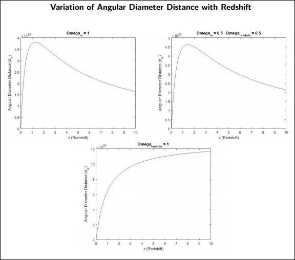
Points to Remember
If we know a sources size, its angular width will tell us its distance from the observer.
Proper distance is the distance that photons travel from the source to us.
Comoving distance is the distance between objects in a space which doesnt expand.
Cosmology - Luminosity Distance
As discussed in the previous chapter, the angular diameter distance to a source at red shift z is given by −
$$d_\wedge (z_{gal}) = \frac{c}{1+z_{gal}}\int_{0}^{z_{gal}} \frac{1}{H(z)}dz$$
$$d_\wedge(z_{gal}) = \frac{r_c}{1+z_{gal}}$$
where $r_c$ is comoving distance.
The Luminosity Distance depends on cosmology and it is defined as the distance at which the observed flux f is from an object.
If the intrinsic luminosity $d_L$ of a distant object is known, we can calculate its luminosity by measuring the flux $f$ which is determined by −
$$d_L(z) = \sqrt{\frac{L}{4\pi f}}$$
The Photon Energy gets red shifted.
$$\frac{\lambda_{obs}}{\lambda_{emi}} = \frac{a_0}{a_e}$$
where $\lambda_{obs}, \lambda_{emi}$ are observed and emitted wave lengths and $a_0, a_e$ are corresponding scale factors.
$$\frac{\Delta t_{obs}}{\Delta t_{emi}} = \frac{a_0}{a_e}$$
where $\Delta_t{obs}$ is observed as the photon time interval, while $\Delta_t{emi}$ is the time interval at which they are emitted.
$$L_{emi} = \frac{nhv_{emi}}{\Delta t_{emi}}$$
$$L_{obs} = \frac{nhv_{obs}}{\Delta t_{obs}}$$
$\Delta t_{obs}$ will take more time than $\Delta t_{emi}$ because the detector should receive all the photons.
$$L_{obs} = L_{emi}\left ( \frac{a_0}{a_e} \right )^2$$
$$L_{obs} < L_{emi}$$
$$f_{obs} = \frac{L_{obs}}{4\pi d_L^2}$$
For a non-expanding universe, luminosity distance is same as the comoving distance.
$$d_L = r_c$$
$$\Rightarrow f_{obs} = \frac{L_{obs}}{4\pi r_c^2}$$
$$f_{obs} = \frac{L_{emi}}{4 \pi r_c^2}\left ( \frac{a_e}{a_0} \right )^2$$
$$\Rightarrow d_L = r_c\left ( \frac{a_0}{a_e} \right )$$
We are finding luminosity distance $d_L$ for calculating luminosity of emitting object $L_{emi}$ −
Interpretation − If we know the red shift z of any galaxy, we can find out $d_A$ and from that we can calculate $r_c$. This is used to find out $d_L$.
If $d_L ! = r_c(a_0/a_e)$, then we cant find Lemi from $f_{obs}$.
The relation between Luminosity Distance $d_L$ and Angular Diameter Distance $d_A.$
We know that −
$$d_A(z_{gal}) = \frac{d_L}{1+z_{gal}}\left ( \frac{a_0}{a_e} \right )$$
$$d_L = (1 + z_{gal})d_A(z_{gal})\left ( \frac{a_0}{a_e} \right )$$
Scale factor when photons are emitted is given by −
$$a_e = \frac{1}{(1+z_{gal})}$$
Scale factor for the present universe is −
$$a_0 = 1$$
$$d_L = (1 + z_{gal})^2d_\wedge(z_{gal})$$
Which one to choose either $d_L$ or $d_A$?
For a galaxy of known size and red shift for calculating how big it is, then $d_A$ is used.
If there is a galaxy of a given apparent magnitude, then to find out how big it is, $d_L$ is used.
Example − If it is given that two galaxies of equal red shift (z = 1) and in the plane of sky they are separated by 2.3 arc sec then what is the maximum physical separation between those two?
For this, use $d_A$ as follows −
$$d_A(z_{gal}) = \frac{c}{1+z_{gal}}\int_{0}^{z_{gal}} \frac{1}{H(z)}dz$$
where z = 1 substitutes H(z) based on the cosmological parameters of the galaxies.
Points to Remember
Luminosity distance depends on cosmology.
If the intrinsic luminosity $d_L$ of a distant object is known, we can calculate its luminosity by measuring the flux f.
For a non-expanding universe, luminosity distance is same as the comoving distance.
Luminosity distance is always greater than the Angular Diameter Distance.
Cosmology - Type 1A Supernovae
For any given redshift (z), we have two values for the distance −
- Angular Diameter Distance (dA)
- Luminosity Distance (dL)
There is no unique definition of cosmological distance in the universe. The choice of the distance depends on the purpose and convenience of application.
To test the predicted trend of how angular size of an object varies with redshift, a standard size yardstick is needed in the sky. This should be an object which −
is very luminous, so that it can be detected at z > 1.
is very large, so that we can resolve its angular size.
has not morphologically evolved over cosmologically significant time (z ∼ 1 corresponds to a look back time of about 7 Gyr).
Some objects (like cD galaxies) satisfy the first two criteria. But almost every object is found to morphologically evolve with time. In general, astrophysical objects (extended sources) tend to be intrinsically smaller in the past because they are still forming.
Luminosity Distance
Luminosity distance depends on cosmology. The dependence of luminosity distance on cosmology makes it a useful measure of the cosmological parameters.
The cosmological parameters can be estimated if we can find a standard candle that does not intrinsically evolve and exists from the local to the high redshift universe.
A standard candle is one which does not differ in its luminosity from source to source. The premise is that any difference in the estimated luminosity of standard candles has to be due to cosmology. One such candle is Type Ia Supernovae.
Type 1a Supernovae (SNe)
These are the result of explosion of a white dwarf after sufficient mass accretion from its companion, a red giant or similar main sequence star, in a binary system. After the red giant comes closer than the Roche lobe distance of the White dwarf, the mass transfer begins and eventually the white dwarf explodes giving out huge amount of energy, leaving no core behind. These are called Type 1a Supernovae. The typical rate of Type 1a Supernovae explosion in a galaxy is 1 per century.
The search for Type 1a SNe has been going on with different teams −
- High z Supernova Search Team (Brian Schmidt, Adam Reiss et al.)
- Supernova Cosmology Project (Saul Perlmutter et al.)
There has been another research team called Carnegie Supernovae Project who has given similar results.
The similarity of results from different teams show the cosmological nature of Type 1a SNe. Hence, they are efficient standard candles.
Points to Remember
There is no unique definition of cosmological distance in the universe.
Angular Diameter Distance and Luminosity Distance are the most used.
A standard candle is the one which does not differ in its luminosity from source to source.
Type 1a SNe satisfies the criteria of being a standard candle.
Cosmology - Cosmic Microwave Background
The CMB (Cosmic Microwave Background) essentially is constituted by the photons of the time when matter and radiation was in equilibrium. By the 1920s, the idea of an expanding universe was accepted and could answer several questions. But questions about the abundance of heavier elements and the abundance were left unanswered. Moreover, the expanding universe implied that the density of matter should decrease down to 0.
In 1948, George Gammow and Ralph Alpher explained the Origin of heavier elements and the abundance using Big Bang. They along with Robert Herman predicted the existence of Relict Radiation or radiation remaining from the Big Bang. The predicted temperature for this remnant radiation was between 50-6 K. In 1965, Robert Dicke, Jim Peebles and David Wilkinson along with the Amo Perizias Research Group experimentally detected the CMB.
The early universe was very hot and the energy was too high for the matter to remain neutral. Hence, matter was in the ionized form - Plasma. The Radiation (photons) and Matter (plasma) interacted mainly through the following three processes.
Compton Scattering − (Major Interaction Process) Inelastic scattering between high energy photon and low energy charged particle.
Thomson Scattering − Elastic scattering of photon by a free charged particle.
Inverse Compton Scattering − High energy charged particle and low energy photon. These interactions finally resulted in matter and radiation being in Thermal equilibrium.
Thermal Equilibrium
In Thermal equilibrium, the radiation obeys the Planck Distribution of Energy,
$$B_v(T) = \frac{2hv^3}{c(e^{hv/k_BT}-1)}$$
During this time, due to the highly frequent interactions, the mean free path of photons was very small. The universe was Opaque to radiation. The early universe was radiation dominated. The universe evolved in such a way that matter and radiation reached Thermal Equilibrium and their energy density became equal. This can be seen from the graph showing evolution of density with the scale factor. Let us find out the scale factor (time) (a(t)) at which the matter and the radiation reached equilibrium.
$$\rho_m \propto \frac{1}{a^3}, \: \rho_r \propto \frac{1}{a^4}$$
$$\frac{\rho_{m,t}}{\rho_{r,t}} = \frac{\Omega_{m,t}}{\Omega_{r,t}} = \frac{\Omega_{m,0}}{\Omega_{r,0}}a(t)$$
At equilibrium,
$$\frac{\rho_{m,t}}{\rho_{r,t}} = \frac{\Omega_{m,t}}{\Omega_{r,t}} = 1$$
$$\Rightarrow \frac{\Omega_{m,0}}{\Omega_{r,0}}a(t) = 1 \: \Rightarrow a(t) = 2.96 \times 10^{-4}$$
using $\Omega_{m,0} = 0.27$ and $\Omega_{r,0} = 8 \times 10^{5}$. The red shift corresponding to this scale factor is given by −
$$z = 1/a(t)-1 \approx 3375$$
The energy density of the radiation went down due to the expansion of the universe. Thus the universe started to cool down. As the energy of the photons started to decrease, neutral atoms started to form. Thus, around a redshift of 1300, neutral Hydrogen started to form. This era had a temperature close to 3000K.
The interaction between matter and radiation became very infrequent and thus the universe started becoming transparent to radiation. This time-period is called Surface of last scattering as the mean free path of the photons became very large due to which hardly any scattering took place after this period. It is also called as Cosmic Photosphere.
Points to Remember
CMB is constituted by the photons of the time when matter and radiation was in equilibrium.
The early universe was very hot and the energy was too high for matter to remain neutral, so it existed as ionized matter-Plasma.
Compton Scattering, Thomson Scattering, Inverse Compton Scattering were the 3 matter-radiation interaction processes then.
Universe evolved such that matter and radiation reached Thermal equilibrium.
CMB Temperature at Decoupling
We should first understand what characterizes the decoupling. We know that energies were much higher to such an extent that matter existed only in the form of Ionized Particles. Thus, at decoupling and recombination epochs, the energy had to drop to permit the ionization of hydrogen. An approximate calculation can be made to the estimation of temperature at the time of decoupling.
This has been performed as follows −
First, consider only the ionization of ground state hydrogen.
$$hv \approx k_BT$$
$$\therefore T \approx \frac{hv}{k_B}$$
For ionization of the ground state hydrogen, h is 13.6 eV and kB is the Boltzmann Constant 8.61 × 10⁵ eV/K that reveals the temperature to be 1.5 × 10⁵ kelvin.
This essentially tells us that if the temperature is below 1.5 × 10⁵ K, the neutral atoms can begin to form.
We know that the ratio of photons to baryons is about 5 × 10¹⁰. Hence even at the tail of the graph where the number of photons reduces, there will still be sufficient photons to ionize the hydrogen atoms. Moreover, recombination of electron and proton does not guarantee a ground state hydrogen atom. Excited states require lesser energy for ionization. Hence a disciplined statistical analysis should be performed case by case to obtain an accurate value. Computations set the temperature to be around 3000K.
For explanations sake, we consider the case of exciting hydrogen into the first excited state. The general expression for the ratio of the number of photons with energy more than ΔE, Nγ (> ΔE) to the total number of photons Nγ is given by −
$$\frac{N_\gamma(> \Delta E)}{N_\gamma} \propto e^{\frac{-\Delta E}{kT}}$$
For the case of exciting hydrogen to the first excited state, ΔE is 10.2 eV. Now, if we consider a highly conservative number of at least 1 photon with energy more than 10.2 for every baryon (keeping in mind that the ratio is 5 × 10¹⁰, we obtain temperature from the equation 3 as 4800 K (Inserted Nγ(> ΔE) = Np).
This is the temperature to create a population of neutral hydrogen atoms in the first excited state. The temperature to ionize this is significantly lesser. Thus, we obtain a better estimate than 1.5 × 10⁵ K that is closer to the accepted value of 3000 K.
Redshift Temperature Relationship
To understand the relationship between redshift and temperature, we employ the following two methods as described below.
Method 1
From Wiens Law, we know that
$$\lambda_mT = constant$$
To relate this to the redshift, we use −
$$1+z = \frac{\lambda_0}{\lambda_e}$$
As $_oT_o = _eT(z)$, we get −
$$T(z) = T_0\frac{\lambda_0}{\lambda_e} = T_0(1+z)$$
Setting To as the current value 3K, we can get temperature values for a given redshift.
Method 2
In terms of frequency, we know −
$$v_0 = \frac{v_e}{1+z}$$
$$B_vdv = \frac{2hv^3}{c^2} \frac{dv}{e^{hv/kT}-1}$$
This tells us about the net energy of the photons for an energy interval and h is the energy of a single photon. Hence, we can obtain the number of photons by Bd/h.
If $n_{o}$ is for present and $n_{e}$ for emitted, we get −
$$\frac{n_{v_e}}{n_{v_0}} = (1+z)^3$$
On simplification, we get,
$$n_{v_0} =\frac{2v_c^2}{c^2}\frac{dv_c}{e^{hv/kT}-1}\frac{1}{(1+z)^3}=\frac{2v_0^2}{c^2}\frac{dv_c}{e^{hv/kT}-1}$$
This gives us the Wiens Law again and thus it can be concluded that −
$$T(z) = T_0\frac{\lambda_0}{\lambda_e} = T_0(1+z)$$
Points to Remember
- The early universe was very hot, ∼ 3000K.
- Current measurements reveal the universes temperature to be close to 3K.
- The further back we go in time, the temperature increases proportionally.
Anisotropy of CMB Radiation & Cobe
In this chapter, we will discuss the anisotropy of CMB Radiation and COBE, i.e., Cosmic Background Explorer.
Primary Anisotropies in the CMB
To understand the observations from space and the primary anisotropies in the Cosmic Microwave Background Radiation, let us take the following equations and understand it as shown below.
CMB Photon Number Density (nγ,0)
$$n_{\gamma,0} = \frac{Total \: energy \: density}{Characteristic \: energy \:of \:Photons}$$
$$n_{\gamma,0} = \frac{aT_0^4}{k_BT_0}$$
Where $k_B$ is Boltzmann Constant and $T_0$ is the present temperature of the universe.
Using the present temperature $(T_0)$ as 2.7 K, we get the current CMB photon number density as 400 cm3.
The cosmic stellar photon number density is much smaller (∼= 103 cm3) over large scales.
Baryon to Photon ratio (η)
If the stellar contributions from galaxies, which get mixed with CMB, are negligible, the baryon to proton ratio is −
$$\eta = \frac{n_{b,0}}{n_{\gamma,0}}$$
The present value is ∼5 1010. Since both photon and baryon number densities are proportional to a3, then η doesnt evolve with time.
Energy Density
As opposed to the number density, the matter energy density is more dominated than photon energy density at present.
The Energy density of baryonic matter = $\rho_{b,0}c^2 = 0.04\rho_cc^2 = 2 10^{9} ergcm^{3}$. While, the Energy density of radiation = $aT_0^4 = 4 \times 10^{13}ergcm{3}$.
Isotropy of CMB Radiation
Penzias and Wilson found the CMB to be isotropic within the limits of observations. The limits are low angular resolution and sensitivity of instruments. They made observations from earth, due to this, observations cannot be made through all the spectrum as water vapor in the atmosphere absorbs many wavelengths ranging from 1mm to 1m. So, CMB cant be asserted as a spectrum.
The CMB is thought to be rotationally invariant (isotropic). Since there existed a time when matter and radiation were in equilibrium, then the formation of structures in the universe is unexplainable. Since the distribution of matter is not isotropic but is clumped together like a cosmic web with huge voids in between, CMB is thought to have an extragalactic origin.
But, as the observations from the space began, anisotropies in the CMB were found, which lead to the reasoning that these anisotropies in matter lead to the formation of structures.
Observation of CMB Radiation from Space
The main satellites which were launched to observe the CMB were −
Cosmic Microwave Background Explorer (COBE, 1989)
Wilkinson Microwave Anisotropy Probe (WMAP, 2001) and
Planck (2009).
COBE (Cosmic Background Explorer)
COBE mainly had two instruments. They were Far InfraRed Absolute Spectrometer (FIRAS) and Differential Microwave Radiometers (DMR Antennas). FIRAS measures intensity of the CMB as a function of wavelength along any specific direction. Whereas, DMR has 3 antennas to measure the difference in intensity of CMB from three different directions. The following pointers give us some more information on FIRAS and DMR.
CMB observations from FIRAS show that the CMB radiation corresponds to black body spectrum at T = 2.72528±0.00065 K.
The DMR measures three frequencies (31.5 GHz, 53 GHz, 90 GHz) in all directions in the sky.
The red batman symbol in the DMR observations is noise from foreground emission (galactic diffused synchrotron emission).
The intensity variations in the observations correspond to temperature variations. The presence of hot and cold spots proves that the CMB radiation is anisotropic.
This anisotropy must be present at decoupling time as there are no distortions in CMB. So, matter should have some pockets with higher density than that of the others.
COBE Results
The CMB spectrum (intensity as a function of energy) is nearly a perfect black body corresponding to T = 2.7 K. The specific intensity of the CMB radiation is nearly the same for all directions. Confirmation that universe is isotropic at large scales (validates our assumption of cosmological principle).
Analysis of the data showed that there are temperature anisotropies (fluctuations) in the CMB spectrum at the resolution of COBE (DMR).
Resolution of COBE, WMAP, Planck
The DMR instrument on-board COBE had a limiting (maximum) spatial resolution of ∼ 7 degrees.
Wilkinson Microwave Anisotropy Probe (WMAP) had an average resolution of ∼ 0.7 degrees.
Planck satellite has an angular resolution of ∼ 10 arc-minute.
Points to Remember
Cosmic stellar photon number density is much smaller than the CMB photon number density.
We live in a matter dominated universe, since matter energy density is higher than the photon energy density.
COBE, WMAP, Planck are efforts to measure and quantify anisotropies in the CMB.
The formation of structure in the universe is a result of CMB anisotropies.
Cosmology - Modelling the CMB Anisotropies
When we look at the refined, corrected all sky CMB map, there is a lot of foreground contamination, which is a kind of anisotropy in these maps. We can see that these foreground emissions are from the milky way galaxy. The intensity of CMB is high along the plane of galactic plane and reduces in intensity as we move away. In these, we can observe secondary anisotropies, which are synchrotron emissions from the galaxy. These emissions make up the foreground contamination. To look at the CMB emission from the sky, we need to subtract these foreground emissions.
The following image shows the CMB with foreground emissions.
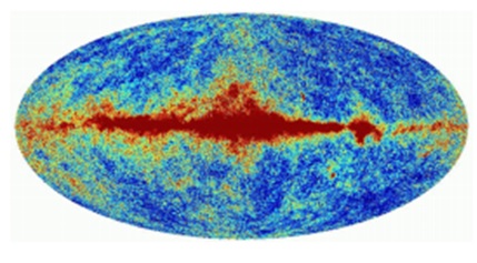
Dipole Anisotropy
There is another kind of anisotropy, which was found in the CMB all sky map, it is called as Dipole Anisotropy. It is not associated with the early universe. This can be represented using spherical harmonic functions. If there is a pattern on spherical surface and we want to map it using mathematical functions, we can do so using trigonometric functions. So, when we map, it can be a monopole same at every direction, or a dipole flips properties when rotated by 180 degrees. Similarly, we have quadrupole and so on. For a complex pattern, it can be expressed as the sum of these monopole, dipole, quadrupole, etc.
The CMB is modelled in such a manner that one of the major sources of anisotropy in the all sky map is this dipole anisotropy, but it is not primordial modelling of CMB. This can be seen in the image below.
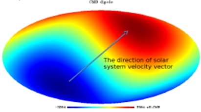
The dipole direction we get to see is not any random direction. Dipole anisotropy has a direction. We see the CMB intensity along a specific direction. This direction is due to the solar system velocity vector. The velocity of earth can be represented with respect to sun or centre of galaxy. The direction in which earth is moving, we observe a Blueshift and Redshift and the dipole lies along this direction.
The above image has a typical dipole appearance because our Galaxy is moving in a specific direction. The result is one side of the sky will appear Redshifted and the other side of the sky will appear Blueshifted. In this case, Redshifting means the photons are longer in wavelength = cooler (so backwards from their name, they look blue in the above diagram).
We can say, the earth is moving in some specific direction with respect to sun/galactic centre/ CMB in the sky at a given instant. Then, if we look at any angle and measure the temperature for CMB, it would be different. This is because, we are measuring photons which are either Blueshifted or Redshifted and depends on the line of sight of photons in the sky.
Points to Remember
The foreground contamination in CMB all sky map is called anisotropy of CMB.
These emissions are from our own milky way galaxy.
The 2 types of anisotropies are: Dipole Anisotropy and Angular Power Spectrum Anisotropy.
Dipole anisotropy is in a specific direction, whereas Angular Power Spectrum anisotropy is spread everywhere.
Horizon Length at the Surface of Last Scattering
Horizon length is the distance travelled by light photons from The Big Bang to The Recombination Era. The 1st peak of the angular spectrum is at θ = 1 (l = 180), which is a very special length scale.
The proper distance between two points is given by −
$$r_p = \int_{0}^{t}cdt$$
When we take the time frame of t = 0 to t = trec, then
$$r_H = \int_{0}^{t_{rec}}cdt$$
Where $r_H$ is the proper horizon distance.
Now, we know that −
$$\dot{a} = \frac{\mathrm{d} a}{\mathrm{d} t}$$
$$dt = \frac{da}{\dot{a}}$$
When t = 0, a = 0.
Then $t = t_{rec}, a = a_0 / (1 + z_{rec})$.
Hence, we can write,
$$r_H(z_{rec})=\int_{0}^{a_{rec}} c\frac{da}{aH}$$
$$H(a_{rec}) = H(z_{rec}) = H_0\sqrt{\Omega_{m,0}}a^{-3/2}$$
During the Recombination period universe was matter dominated. i.e., rad << Ωmatter. Therefore, the term radiation is dropped.
$$r_H(z_{rec}) = \frac{c}{H_0\sqrt{\Omega_{m,0}}}\int_{0}^{a_{rec}} \frac{da}{a^{-1/2}}$$
$$r_H(z_{rec}) = \frac{2c}{3H_0\sqrt{\Omega_{m,0}}}\frac{1}{(1+z_{rec})^{3/2}}$$
$$\theta_H(rec) = \frac{r_H(z_{rec})}{d_A(z_{rec})}$$
Which is equal to 0.5 degrees, if we put all the known values in the equation.
The Electromagnetic radiation is opaque from the surface of last scattering. Any two points not lying within the horizon of each other need not have the same properties. So, it will give different temperature values.
We can get two points on this surface which did not intersect with each other, which means at one point the universe expanded faster than the speed of light which is the inflationary model for expansion.
Points to Remember
The horizon length is the distance travelled by light photons from The Big Bang to The Recombination Era.
During the Recombination period, the universe was matter dominated.
Electromagnetic radiation is opaque from the surface of last scattering.
Cosmology - Extrasolar Planet Detection
Astrobiology is the study of origin, evolution, distribution and future of life in the universe. It is concerned with discovering and detecting Extrasolar Planets.
Astrobiology addresses the following points −
How does life begin and evolve? (biology + geology + chemistry + atmospheric sciences)
Are there worlds beyond earth that are favorable for life? (astronomy)
What would be the future of life on earth?
Astronomy addresses the following points −
How to detect the planetary system around other stars?
One of the method is direct imaging, but it is a very difficult task because planets are extremely faint light sources compared to stars, and what little light comes from them tends to be lost in the glare from their parent star.
Contrast is better when the planet is closer to its parent star and hot, so that it emits intense infrared radiation. We can make images in the infrared region.
Techniques for Extrasolar Planet Detection
The most efficient techniques for extrasolar planet detection are as follows. Each of these are also explained in detail in the subsequent chapters.
Radial Velocity Method
It is also called as the Doppler method. In this −
The star planet system revolves around their barycenter, star wobbles.
Wobbling can be detected by
Periodic Red/Blue shifts. Astrometry - measuring the objects in the sky very precisely.
Transit Method
Transit Method (Kepler space telescope) is used to find out the size. The dip in brightness of star by planet is usually very less, unlike in a binary system.
Direct Imaging
Imaging the planet using a telescope.
Let us look at a case study done on Radial Velocity Method.
Case Study
This case study is on the Circular orbit and the plane of the orbit perpendicular to the plane of the sky. The time taken by both around the barycenter will be same. It will be equal to the time difference between two Redshift or Blueshift.
Consider the following image.
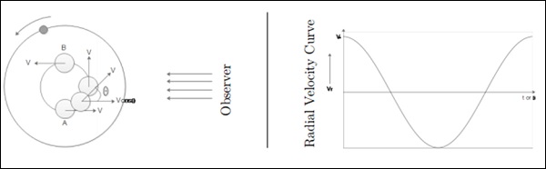
At A and C full velocity is measured. At C, velocity is zero.
Vrmax = V* is the true velocity of the star.
P is the time-period of the star as well as the planet.
θ is the phase of orbit.
Star Mass - M*, Orbit radius a*, planet mass mp.
From center of mass equation,
$$m_p a_p = M_\ast a_\ast$$
From equation of velocity,
$$V_\ast = \frac{2\pi a_\ast}{P}$$
$$\Rightarrow a_\ast = \frac{PV_\ast}{2\pi}$$
From Keplers Law,
$$P^2 = \frac{4\pi^2a_p^3}{GM_\ast}$$
$$\Rightarrow a_p = \left ( \frac{P^2GM_\ast}{4\pi^2} \right)^{1/3}$$
From the above equations, we get −
$$\Rightarrow m_p = \left( \frac{P}{2\pi G} \right)^{1/3}M_\ast^{2/3}V_\ast$$
We get: $m_p, a_p$ and $a_\ast$.
The above equation is biased towards most massive planets close to the star.
Points to Remember
Astrobiology is the study of origin, evolution, distribution and future of life in the universe.
Techniques to detect the extrasolar planets are: Radial Velocity Method, Transit Method, Direct Imaging, etc.
Wobbling can be detected by periodic red/blue shifts and Astrometry.
The Radial Velocity Method is biased towards detecting massive planets close to the star.
Cosmology - Radial Velocity Method
In the previous chapter, the Radial Velocity Method for the case in which the orbital plane and the plane of sky are perpendicular was discussed for circular orbits. Here, we deal with one more case, when the orbital plane and the plane of sky are not perpendicular for circular orbits.
When the orbital plane is at an angle with respect to the plane of sky (not perpendicular), we have the following situation −
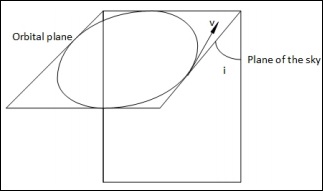
In this case, when they were perpendicular, we had two points at which we could measure the true velocity. But here, that is not possible. At all points, we can measure only a component of the true velocity, v.
$$v_r = v \:sin(i)cos(\theta)$$
where θ is the phase of the orbit which is a time-dependent quantity. The inclination angle i on the other hand, is time-independent. Hence,
$$(v_r)_{max} = v\: sin(i)$$
The observed radial velocity curve will be of the following form −
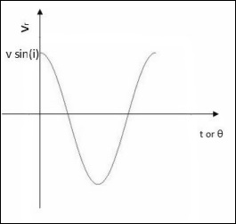
When the orbital plane is perpendicular to the sky −
$$m_p = \left ( \frac{P}{2\pi G} \right )^{\frac{1}{3}}(M_\ast)^{\frac{2}{3}}v$$
where mp, P, G, M∗ are mass of the planet, orbital period, universal gravitational constant and mass of the star respectively. But in this case, we should modify it as follows −
$$m_psin(i) = \left ( \frac{P}{2\pi G} \right )^{\frac{1}{3}} (M_\ast)^{\frac{2}{3}}(v_r)_{max}$$
But, finding the value of i is a difficult task. We can impose certain constraints on the value of i using transit method. The passage of the planet between the star and the Earth is called a transit. We can obtain the light curve by observing a transit and a significant dip in observed flux of a light curve implies that i is close to 90 degrees. If such conditions are not satisfied, we cannot have any idea on the value of i. Then the value of mp that we find can serve as a lower limit for the mass of the planet, since it is actually mp sin(i) and sin(i) ≤ 1.
To conclude, the Radial velocity method is more convenient than the transit method because radial velocity can be measured at any time but transit measurements can be made only during the transit which may not last for long.
Points to Remember
Finding inclination of the planets orbit is not achieved by Radial Velocity method.
Radial Velocity Method is better than the Transit Method because radial velocity can be measured always unlike transits.
Transits are short-lived and very easy to miss.
Cosmology - Transit Method
The Transit Method (Kepler Space Telescope) is used to find out the size. The dip in brightness of a star by a planet is usually very less unlike a binary system.
F0 is flux of the star before the planet occults it.
F1 is the flux after the entire planet is in front of star.
The following image will be used for all the calculations.
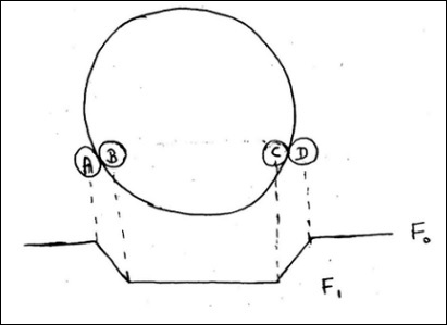
$$\frac{F_0 - F_1}{F_0} = \frac{\pi r_p^{2}}{\pi R^2_\ast}$$
$$\frac{\Delta F}{F} \cong \frac{r^2_p}{R^2_\ast}$$
$$\left ( \frac{\Delta F}{F} \right )_{earth} \cong 0.001\%$$
$$\left ( \frac{\Delta F}{F} \right )_{jupiter} \cong 1\%$$
This is not easy to achieve by ground based telescope. It is achieved by the Hubble telescope.
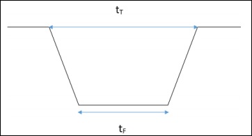
Here, $t_T$ is time between position A and D and $t_F$ is time between position B and C.
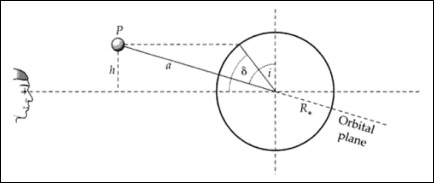
The geometry of a transit related to the inclination i of the system. Transit latitude and inclination are interchangeable.
From the above images, we can write −
$$\frac{h}{a} = cos(i)$$
$$\frac{h}{R_\ast} = sin(\delta)$$
$$cos(i) = \frac{R_\ast sin(\delta)}{a}$$
$$y^2 = (R_\ast + R_p)^2 - h^2$$
$$y = [(R_\ast + R_p)^2 - h^2]^{\frac{1}{2}}$$
$$sin(\theta) = \frac{y}{a}$$
$$\theta = sin^{-1}\left [ \frac{(R_\ast + R_p)^2 - a^2cos^2(i)}{a^2} \right ]^{\frac{1}{2}}$$
$$t_T = \frac{P}{2\pi} \times 2\theta$$
Here, $t_T$ is the fraction of a time-period for which transit happens and (2θ/2π) is fraction of angle for which the transit happens.
$$sin(\frac{t_T\pi}{P}) = \frac{R_\ast}{a}\left [ \left ( 1+ \frac{R_p}{R_\ast}\right )^2 - \left ( \frac{a}{R_\ast}cos(i)\right )^2 \right ]^{\frac{1}{2}}$$
Usually, a >> R∗ >> Rp. So, we can write −
$$sin(\frac{t_T\pi}{P}) = \frac{R_\ast}{a}\left [ 1- \left ( \frac{a}{R_\ast}cos(i) \right )^2\right ]^{\frac{1}{2}}$$
Here, P is the duration between two successive transits. The transit time is very less compared to the orbital time-period. Hence,
$$t_T = \frac{P}{\pi}\left [ \left ( \frac{R_\ast}{a}\right )^2 - cos^2(i)\right ]^{\frac{1}{2}}$$
Here, tT, P, R∗ are the observables, a and i should be found out.
Now,
$$sin(\frac{t_F\pi}{P}) = \frac{R_\ast}{a}\left [\left (1 - \frac{R_p}{R_\ast} \right )^2 - \left ( \frac{a}{R_\ast}cos\:i \right )^2\right ]^{\frac{1}{2}}$$
where, $y^2 = (R_\ast R_p)^2 h^2$.
Let,
$$\frac{\Delta F}{F} = D = \left ( \frac{R_p}{R_\ast} \right )^2$$
Now, we can express,
$$\frac{a}{R_\ast} = \frac{2P}{\pi} D^{\frac{1}{4}}(t^2_T - t^2_F)^{-\frac{1}{2}}$$
For the main sequence stars,
$$R_\ast \propto M^\alpha_\ast$$
$$\frac{R_\ast}{R_0} \propto \left ( \frac{M_\ast}{M_0}\right )^\alpha$$
This gives R∗.
Hence, we get value of a also.
So, we get Rp, ap and even i.
For all this,
$$h \leq R_\ast + R_p$$
$$a\: cos\: i \leq R_\ast + R_p$$
For even ~89 degrees, the transit duration is very small. The planet must be very close to get a sufficient transit time. This gives a tight constraint on i. Once we get i, we can derive mpfrom the radial velocity measurement.
This detection by the transit method is called as chance detection, i.e., probability of observing a transit. Transit probability (probability of observing) calculations are shown below.
The transit probability is related to the solid angle traced out by the two extreme transit configurations, which is −
$$Solid \: angle \:of \:planet \: = 2\pi \left ( \frac{2R_\ast}{a} \right )$$
As well as the total solid angle at a semi-major axis a, or −
$$Solid \:angle \:of \:sphere \: =\: 4\pi$$
The probability is the ratio of these two areas −
$$= \: \frac{area \:of\: sky \: covered \:by\: favourable \: orientation}{area\: of\: sky \:covered\: by\: all\: possible\: orientation\: of\: orbit}$$
$= \frac{4\pi a_pR_\ast}{4\pi a^2_p} = \frac{R_\ast}{a_p}$ $\frac{area\: of\: hollow \: cyclinder}{area\: of\: sphere}$
This probability is independent of the observer.
Points to Remember
- The Transit Method (Kepler Space Telescope) is used to find out the size.
- Detection by Transit Method is a chance detection.
- The planet must be very close to get sufficient transit time.
- Transit probability is related to the solid angle of planet.
- This probability is independent of observer frame of reference.
Cosmology - Exoplanet Properties
First direct image of an extrasolar planet, in 2004, was of a planet of mass 3-10 Mjupiter orbiting around a brown dwarf (2M1207) with a mass of 25 Mjupiter. Techniques like Radial velocity, Transit, Gravitational microlensing, Imaging, Astrometry, etc., has been used for detection of exoplanets. The number of detections have been increasing every year.
Until around 2010, the Radial velocity method was used extensively, but now most of the detections are done by the Transit method. There was a spike in the number of detections in 2014, which was when Kepler Space Telescope (KST) started giving the results.
A mass-period distribution shows that the Radial velocity method is more biased towards detection of massive planets with a larger period, whereas using the Transit method, planets with lower period are only detected as shown in the following image (Courtesy: NASA Exoplanet Archive).
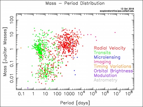
There is a colossal increase in the number of detection of smaller mass planets since the advent of KST. This is evident from the figure given below. The planets detected by KST are divided into two groups: hot massive planets called Hot Jupiters and lower mass planets called Hot Super Earths (as they are more massive than Earth).
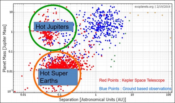
When we plot the number of extrasolar planets detected versus distance to them, we find that most of these planets are within 2kpc, which is well within our galaxy. Maybe the planets are not so uncommon in the universe, since our detection is limited to only certain type of planets in a very small part of the universe.
Planets are formed from circumstellar disc or proto planetary disc. If planets are formed as a by-product during star formation, maybe the number planets in the universe exceeds the number of stars in universe!!
Habitable Zones
A Habitable Zone can be defined as the zone around the star where water can exist in its liquid form. Consider a planet at distance $a_p$ from the star as shown in the following figure. A simple method for calculating the temperature of the planet is described as follows.
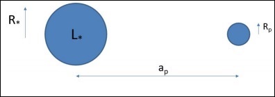
$$\left ( \frac{L_\ast}{4\pi a^2_p} \right )\pi R^2_p(1 - A) = 4\pi R^2_p \sigma T^4_p$$
and
$$\frac{L_\ast}{4\pi R^2_\ast} = \sigma T^4_\ast$$
$$\therefore T_p = (1 - A)T_\ast \sqrt{\frac{R_\ast}{2a_p}}$$
In our case substituting
Lsun = 3.83 x 1026
ap = 1.5 ∗ 1011 and
A = 0.3
Will give $T_{Earth} = 255K$. The actual calculation is very involved which includes cloud physics. The Habitable zone in our solar system lies between 0.9 AU and 1.7 AU.
The Suns luminosity was found to be increasing with time because of the decreasing gas pressure. It was 30% less bright when it started burning hydrogen. This would result is shift of habitable zone away from the Sun. Since Earth is near the inner edge of the Habitable zone, maybe one day it will move out of the zone!
Continuously Habitable Zone
In short it is termed as CHZ can be defined as the region in which liquid water can exist over the entire Main Sequence lifetime of a star. The KST has detected many extrasolar planets which do lie in the habitable zone.
A bio-signature is any substance such as an element, isotope, molecule, or phenomenon that provides scientific evidence of past or present life. An example is detection of both O2 and CO2 on a planet, which is usually not possible through geological processes alone. This detection is done by analyzing the absorption spectra.
Points to Remember
Techniques like Radial velocity, Transit, Gravitational microlensing, Imaging, Astrometry, etc., have been used for detection of exoplanets.
Radial velocity method is more biased towards detection of massive planets with larger period.
Hot massive planets are called Hot Jupiters and lower mass planets are called Hot Super Earths.
The number of planets in the universe exceeds the number of stars in the universe.
A Habitable zone can be defined as the zone around the star where water can exist in its liquid form.
