- Cosmology - Home
- The Expanding Universe
- Cepheid Variables
- Redshift and Recessional Velocity
- Redshift Vs. Kinematic Doppler Shift
- Cosmological Metric & Expansion
- Robertson-Walker Metric
- Hubble Parameter & Scale Factor
- Friedmann Equation & World Models
- Fluid Equation
- Matter Dominated Universe
- Radiation Dominated Universe
- The Dark Energy
- Spiral Galaxy Rotation Curves
- Velocity Dispersion Measurements of Galaxies
- Hubble & Density Parameter
- Age of The Universe
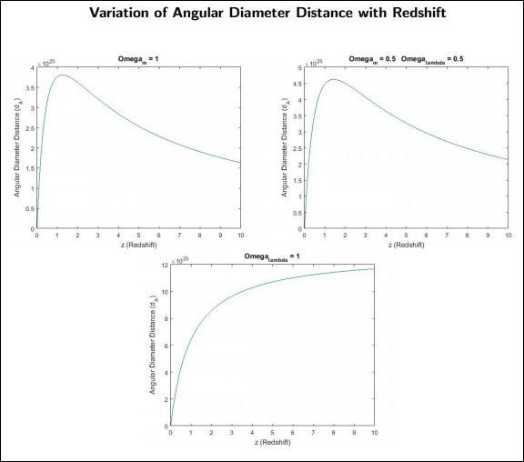
- Angular Diameter Distance
- Luminosity Distance
- Type 1A Supernovae
- Cosmic Microwave Background
- CMB - Temperature at Decoupling
- Anisotropy of CMB Radiation & Cobe
- Modelling the CMB Anisotropies
- Horizon Length at the Surface of Last Scattering
- Extrasolar Planet Detection
- Radial Velocity Method
- Transit Method
- Exoplanet Properties
Cosmology - Angular Diameter Distance
In this chapter, we will understand what the Angular Diameter Distance is and how it helps in Cosmology.
For the present universe −
$\Omega_{m,0} \: = \: 0.3$
$\Omega_{\wedge,0} \: = \: 0.69$
$\Omega_{rad,0} \: = \: 0.01$
$\Omega_{k,0} \: = \: 0$
Weve studied two types of distances till now −
Proper distance (lp) − The distance that photons travel from the source to us, i.e., The Instantaneous distance.
Comoving distance (lc) − Distance between objects in a space which doesnt expand, i.e., distance in a comoving frame of reference.
Distance as a Function of Redshift
Consider a galaxy which radiates a photon at time t1 which is detected by the observer at t0. We can write the proper distance to the galaxy as −
$$l_p = \int_{t_1}^{t_0} cdt$$
Let the galaxys redshift be z,
$$\Rightarrow \frac{\mathrm{d} z}{\mathrm{d} t} = -\frac{1}{a^2}\frac{\mathrm{d} a}{\mathrm{d} t}$$
$$\Rightarrow \frac{\mathrm{d} z}{\mathrm{d} t} = -\frac{\frac{\mathrm{d} a}{\mathrm{d} t}}{a}\frac{1}{a}$$
$$\therefore \frac{\mathrm{d} z}{\mathrm{d} t} = -\frac{H(z)}{a}$$
Now, comoving distance of the galaxy at any time t will be −
$$l_c = \frac{l_p}{a(t)}$$
$$l_c = \int_{t_1}^{t_0} \frac{cdt}{a(t)}$$
In terms of z,
$$l_c = \int_{t_0}^{t_1} \frac{cdz}{H(z)}$$
There are two ways to find distances, which are as follows −
Flux-Luminosity Relationship
$$F = \frac{L}{4\pi d^2}$$
where d is the distance at the source.
The Angular Diameter Distance of a Source
If we know a sources size, its angular width will tell us its distance from the observer.
$$\theta = \frac{D}{l}$$
where l is the angular diameter distance of the source.
θ is the angular size of the source.
D is the size of the source.
Consider a galaxy of size D and angular size dθ.
We know that,
$$d\theta = \frac{D}{d_A}$$
$$\therefore D^2 = a(t)^2(r^2 d\theta^2) \quad \because dr^2 = 0; \: d\phi ^2 \approx 0$$
$$\Rightarrow D = a(t)rd\theta$$
Changing r to rc, the comoving distance of the galaxy, we have −
$$d\theta = \frac{D}{r_ca(t)}$$
Here, if we choose t = t0, we end up measuring the present distance to the galaxy. But D is measured at the time of emission of the photon. Therefore, by using t = t0, we get a larger distance to the galaxy and hence an underestimation of its size. Therefore, we should use the time t1.
$$\therefore d\theta = \frac{D}{r_ca(t_1)}$$
Comparing this with the previous result, we get −
$$d_\wedge = a(t_1)r_c$$
$$r_c = l_c = \frac{d_\wedge}{a(t_1)} = d_\wedge(1+z_1) \quad \because 1+z_1 = \frac{1}{a(t_1)}$$
Therefore,
$$d_\wedge = \frac{c}{1+z_1} \int_{0}^{z_1} \frac{dz}{H(z)}$$
dA is the Angular Diameter Distance for the object.
Points to Remember
If we know a sources size, its angular width will tell us its distance from the observer.
Proper distance is the distance that photons travel from the source to us.
Comoving distance is the distance between objects in a space which doesnt expand.
