- Artificial Neural Network - Home
- Basic Concepts
- Building Blocks
- Learning & Adaptation
- Supervised Learning
- Unsupervised Learning
- Learning Vector Quantization
- Adaptive Resonance Theory
- Kohonen Self-Organizing Feature Maps
- Associate Memory Network
- Hopfield Networks
- Boltzmann Machine
- Brain-State-in-a-Box Network
- Optimization Using Hopfield Network
- Other Optimization Techniques
- Genetic Algorithm
- Applications of Neural Networks
Supervised Neural Networks
As the name suggests, supervised learning takes place under the supervision of a teacher. This learning process is dependent. During the training of ANN under supervised learning, the input vector is presented to the network, which will produce an output vector. This output vector is compared with the desired/target output vector. An error signal is generated if there is a difference between the actual output and the desired/target output vector. On the basis of this error signal, the weights would be adjusted until the actual output is matched with the desired output.
Perceptron
Developed by Frank Rosenblatt by using McCulloch and Pitts model, perceptron is the basic operational unit of artificial neural networks. It employs supervised learning rule and is able to classify the data into two classes.
Operational characteristics of the perceptron: It consists of a single neuron with an arbitrary number of inputs along with adjustable weights, but the output of the neuron is 1 or 0 depending upon the threshold. It also consists of a bias whose weight is always 1. Following figure gives a schematic representation of the perceptron.
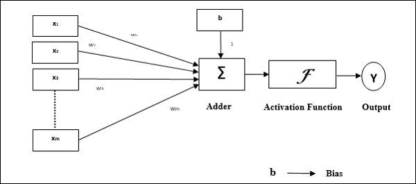
Perceptron thus has the following three basic elements −
Links − It would have a set of connection links, which carries a weight including a bias always having weight 1.
Adder − It adds the input after they are multiplied with their respective weights.
Activation function − It limits the output of neuron. The most basic activation function is a Heaviside step function that has two possible outputs. This function returns 1, if the input is positive, and 0 for any negative input.
Training Algorithm
Perceptron network can be trained for single output unit as well as multiple output units.
Training Algorithm for Single Output Unit
Step 1 − Initialize the following to start the training −
- Weights
- Bias
- Learning rate $\alpha$
For easy calculation and simplicity, weights and bias must be set equal to 0 and the learning rate must be set equal to 1.
Step 2 − Continue step 3-8 when the stopping condition is not true.
Step 3 − Continue step 4-6 for every training vector x.
Step 4 − Activate each input unit as follows −
$$x_{i}\:=\:s_{i}\:(i\:=\:1\:to\:n)$$
Step 5 − Now obtain the net input with the following relation −
$$y_{in}\:=\:b\:+\:\displaystyle\sum\limits_{i}^n x_{i}.\:w_{i}$$
Here b is bias and n is the total number of input neurons.
Step 6 − Apply the following activation function to obtain the final output.
$$f(y_{in})\:=\:\begin{cases}1 & if\:y_{in}\:>\:\theta\\0 & if \: -\theta\:\leqslant\:y_{in}\:\leqslant\:\theta\\-1 & if\:y_{in}\:
Step 7 − Adjust the weight and bias as follows −
Case 1 − if y ≠ t then,
$$w_{i}(new)\:=\:w_{i}(old)\:+\:\alpha\:tx_{i}$$
$$b(new)\:=\:b(old)\:+\:\alpha t$$
Case 2 − if y = t then,
$$w_{i}(new)\:=\:w_{i}(old)$$
$$b(new)\:=\:b(old)$$
Here y is the actual output and t is the desired/target output.
Step 8 − Test for the stopping condition, which would happen when there is no change in weight.
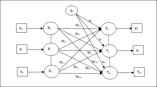
Training Algorithm for Multiple Output Units
The following diagram is the architecture of perceptron for multiple output classes.
Step 1 − Initialize the following to start the training −
- Weights
- Bias
- Learning rate $\alpha$
For easy calculation and simplicity, weights and bias must be set equal to 0 and the learning rate must be set equal to 1.
Step 2 − Continue step 3-8 when the stopping condition is not true.
Step 3 − Continue step 4-6 for every training vector x.
Step 4 − Activate each input unit as follows −
$$x_{i}\:=\:s_{i}\:(i\:=\:1\:to\:n)$$
Step 5 − Obtain the net input with the following relation −
$$y_{in}\:=\:b\:+\:\displaystyle\sum\limits_{i}^n x_{i}\:w_{ij}$$
Here b is bias and n is the total number of input neurons.
Step 6 − Apply the following activation function to obtain the final output for each output unit j = 1 to m −
$$f(y_{in})\:=\:\begin{cases}1 & if\:y_{inj}\:>\:\theta\\0 & if \: -\theta\:\leqslant\:y_{inj}\:\leqslant\:\theta\\-1 & if\:y_{inj}\:
Step 7 − Adjust the weight and bias for x = 1 to n and j = 1 to m as follows −
Case 1 − if yj ≠ tj then,
$$w_{ij}(new)\:=\:w_{ij}(old)\:+\:\alpha\:t_{j}x_{i}$$
$$b_{j}(new)\:=\:b_{j}(old)\:+\:\alpha t_{j}$$
Case 2 − if yj = tj then,
$$w_{ij}(new)\:=\:w_{ij}(old)$$
$$b_{j}(new)\:=\:b_{j}(old)$$
Here y is the actual output and t is the desired/target output.
Step 8 − Test for the stopping condition, which will happen when there is no change in weight.
Adaptive Linear Neuron (Adaline)
Adaline which stands for Adaptive Linear Neuron, is a network having a single linear unit. It was developed by Widrow and Hoff in 1960. Some important points about Adaline are as follows −
It uses bipolar activation function.
It uses delta rule for training to minimize the Mean-Squared Error (MSE) between the actual output and the desired/target output.
The weights and the bias are adjustable.
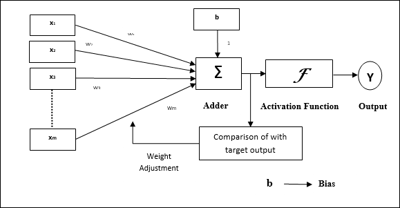
Architecture
The basic structure of Adaline is similar to perceptron having an extra feedback loop with the help of which the actual output is compared with the desired/target output. After comparison on the basis of training algorithm, the weights and bias will be updated.
Training Algorithm
Step 1 − Initialize the following to start the training −
- Weights
- Bias
- Learning rate $\alpha$
For easy calculation and simplicity, weights and bias must be set equal to 0 and the learning rate must be set equal to 1.
Step 2 − Continue step 3-8 when the stopping condition is not true.
Step 3 − Continue step 4-6 for every bipolar training pair s:t.
Step 4 − Activate each input unit as follows −
$$x_{i}\:=\:s_{i}\:(i\:=\:1\:to\:n)$$
Step 5 − Obtain the net input with the following relation −
$$y_{in}\:=\:b\:+\:\displaystyle\sum\limits_{i}^n x_{i}\:w_{i}$$
Here b is bias and n is the total number of input neurons.
Step 6 − Apply the following activation function to obtain the final output −
$$f(y_{in})\:=\:\begin{cases}1 & if\:y_{in}\:\geqslant\:0 \\-1 & if\:y_{in}\:
Step 7 − Adjust the weight and bias as follows −
Case 1 − if y ≠ t then,
$$w_{i}(new)\:=\:w_{i}(old)\:+\: \alpha(t\:-\:y_{in})x_{i}$$
$$b(new)\:=\:b(old)\:+\: \alpha(t\:-\:y_{in})$$
Case 2 − if y = t then,
$$w_{i}(new)\:=\:w_{i}(old)$$
$$b(new)\:=\:b(old)$$
Here y is the actual output and t is the desired/target output.
$(t\:-\;y_{in})$ is the computed error.
Step 8 − Test for the stopping condition, which will happen when there is no change in weight or the highest weight change occurred during training is smaller than the specified tolerance.
Multiple Adaptive Linear Neuron (Madaline)
Madaline which stands for Multiple Adaptive Linear Neuron, is a network which consists of many Adalines in parallel. It will have a single output unit. Some important points about Madaline are as follows −
It is just like a multilayer perceptron, where Adaline will act as a hidden unit between the input and the Madaline layer.
The weights and the bias between the input and Adaline layers, as in we see in the Adaline architecture, are adjustable.
The Adaline and Madaline layers have fixed weights and bias of 1.
Training can be done with the help of Delta rule.
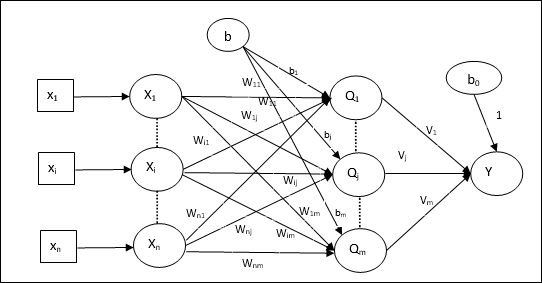
Architecture
The architecture of Madaline consists of n neurons of the input layer, m neurons of the Adaline layer, and 1 neuron of the Madaline layer. The Adaline layer can be considered as the hidden layer as it is between the input layer and the output layer, i.e. the Madaline layer.
Training Algorithm
By now we know that only the weights and bias between the input and the Adaline layer are to be adjusted, and the weights and bias between the Adaline and the Madaline layer are fixed.
Step 1 − Initialize the following to start the training −
- Weights
- Bias
- Learning rate $\alpha$
For easy calculation and simplicity, weights and bias must be set equal to 0 and the learning rate must be set equal to 1.
Step 2 − Continue step 3-8 when the stopping condition is not true.
Step 3 − Continue step 4-7 for every bipolar training pair s:t.
Step 4 − Activate each input unit as follows −
$$x_{i}\:=\:s_{i}\:(i\:=\:1\:to\:n)$$
Step 5 − Obtain the net input at each hidden layer, i.e. the Adaline layer with the following relation −
$$Q_{inj}\:=\:b_{j}\:+\:\displaystyle\sum\limits_{i}^n x_{i}\:w_{ij}\:\:\:j\:=\:1\:to\:m$$
Here b is bias and n is the total number of input neurons.
Step 6 − Apply the following activation function to obtain the final output at the Adaline and the Madaline layer −
$$f(x)\:=\:\begin{cases}1 & if\:x\:\geqslant\:0 \\-1 & if\:x\:
Output at the hidden (Adaline) unit
$$Q_{j}\:=\:f(Q_{inj})$$
Final output of the network
$$y\:=\:f(y_{in})$$
i.e. $\:\:y_{inj}\:=\:b_{0}\:+\:\sum_{j = 1}^m\:Q_{j}\:v_{j}$
Step 7 − Calculate the error and adjust the weights as follows −
Case 1 − if y ≠ t and t = 1 then,
$$w_{ij}(new)\:=\:w_{ij}(old)\:+\: \alpha(1\:-\:Q_{inj})x_{i}$$
$$b_{j}(new)\:=\:b_{j}(old)\:+\: \alpha(1\:-\:Q_{inj})$$
In this case, the weights would be updated on Qj where the net input is close to 0 because t = 1.
Case 2 − if y ≠ t and t = -1 then,
$$w_{ik}(new)\:=\:w_{ik}(old)\:+\: \alpha(-1\:-\:Q_{ink})x_{i}$$
$$b_{k}(new)\:=\:b_{k}(old)\:+\: \alpha(-1\:-\:Q_{ink})$$
In this case, the weights would be updated on Qk where the net input is positive because t = -1.
Here y is the actual output and t is the desired/target output.
Case 3 − if y = t then
There would be no change in weights.
Step 8 − Test for the stopping condition, which will happen when there is no change in weight or the highest weight change occurred during training is smaller than the specified tolerance.
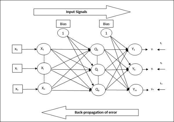
Back Propagation Neural Networks
Back Propagation Neural (BPN) is a multilayer neural network consisting of the input layer, at least one hidden layer and output layer. As its name suggests, back propagating will take place in this network. The error which is calculated at the output layer, by comparing the target output and the actual output, will be propagated back towards the input layer.
Architecture
As shown in the diagram, the architecture of BPN has three interconnected layers having weights on them. The hidden layer as well as the output layer also has bias, whose weight is always 1, on them. As is clear from the diagram, the working of BPN is in two phases. One phase sends the signal from the input layer to the output layer, and the other phase back propagates the error from the output layer to the input layer.
Training Algorithm
For training, BPN will use binary sigmoid activation function. The training of BPN will have the following three phases.
Phase 1 − Feed Forward Phase
Phase 2 − Back Propagation of error
Phase 3 − Updating of weights
All these steps will be concluded in the algorithm as follows
Step 1 − Initialize the following to start the training −
- Weights
- Learning rate $\alpha$
For easy calculation and simplicity, take some small random values.
Step 2 − Continue step 3-11 when the stopping condition is not true.
Step 3 − Continue step 4-10 for every training pair.
Phase 1
Step 4 − Each input unit receives input signal xi and sends it to the hidden unit for all i = 1 to n
Step 5 − Calculate the net input at the hidden unit using the following relation −
$$Q_{inj}\:=\:b_{0j}\:+\:\sum_{i=1}^n x_{i}v_{ij}\:\:\:\:j\:=\:1\:to\:p$$
Here b0j is the bias on hidden unit, vij is the weight on j unit of the hidden layer coming from i unit of the input layer.
Now calculate the net output by applying the following activation function
$$Q_{j}\:=\:f(Q_{inj})$$
Send these output signals of the hidden layer units to the output layer units.
Step 6 − Calculate the net input at the output layer unit using the following relation −
$$y_{ink}\:=\:b_{0k}\:+\:\sum_{j = 1}^p\:Q_{j}\:w_{jk}\:\:k\:=\:1\:to\:m$$
Here b0k is the bias on output unit, wjk is the weight on k unit of the output layer coming from j unit of the hidden layer.
Calculate the net output by applying the following activation function
$$y_{k}\:=\:f(y_{ink})$$
Phase 2
Step 7 − Compute the error correcting term, in correspondence with the target pattern received at each output unit, as follows −
$$\delta_{k}\:=\:(t_{k}\:-\:y_{k})f^{'}(y_{ink})$$
On this basis, update the weight and bias as follows −
$$\Delta v_{jk}\:=\:\alpha \delta_{k}\:Q_{ij}$$
$$\Delta b_{0k}\:=\:\alpha \delta_{k}$$
Then, send $\delta_{k}$ back to the hidden layer.
Step 8 − Now each hidden unit will be the sum of its delta inputs from the output units.
$$\delta_{inj}\:=\:\displaystyle\sum\limits_{k=1}^m \delta_{k}\:w_{jk}$$
Error term can be calculated as follows −
$$\delta_{j}\:=\:\delta_{inj}f^{'}(Q_{inj})$$
On this basis, update the weight and bias as follows −
$$\Delta w_{ij}\:=\:\alpha\delta_{j}x_{i}$$
$$\Delta b_{0j}\:=\:\alpha\delta_{j}$$
Phase 3
Step 9 − Each output unit (ykk = 1 to m) updates the weight and bias as follows −
$$v_{jk}(new)\:=\:v_{jk}(old)\:+\:\Delta v_{jk}$$
$$b_{0k}(new)\:=\:b_{0k}(old)\:+\:\Delta b_{0k}$$
Step 10 − Each output unit (zjj = 1 to p) updates the weight and bias as follows −
$$w_{ij}(new)\:=\:w_{ij}(old)\:+\:\Delta w_{ij}$$
$$b_{0j}(new)\:=\:b_{0j}(old)\:+\:\Delta b_{0j}$$
Step 11 − Check for the stopping condition, which may be either the number of epochs reached or the target output matches the actual output.
Generalized Delta Learning Rule
Delta rule works only for the output layer. On the other hand, generalized delta rule, also called as back-propagation rule, is a way of creating the desired values of the hidden layer.
Mathematical Formulation
For the activation function $y_{k}\:=\:f(y_{ink})$ the derivation of net input on Hidden layer as well as on output layer can be given by
$$y_{ink}\:=\:\displaystyle\sum\limits_i\:z_{i}w_{jk}$$
And $\:\:y_{inj}\:=\:\sum_i x_{i}v_{ij}$
Now the error which has to be minimized is
$$E\:=\:\frac{1}{2}\displaystyle\sum\limits_{k}\:[t_{k}\:-\:y_{k}]^2$$
By using the chain rule, we have
$$\frac{\partial E}{\partial w_{jk}}\:=\:\frac{\partial }{\partial w_{jk}}(\frac{1}{2}\displaystyle\sum\limits_{k}\:[t_{k}\:-\:y_{k}]^2)$$
$$=\:\frac{\partial }{\partial w_{jk}}\lgroup\frac{1}{2}[t_{k}\:-\:t(y_{ink})]^2\rgroup$$
$$=\:-[t_{k}\:-\:y_{k}]\frac{\partial }{\partial w_{jk}}f(y_{ink})$$
$$=\:-[t_{k}\:-\:y_{k}]f(y_{ink})\frac{\partial }{\partial w_{jk}}(y_{ink})$$
$$=\:-[t_{k}\:-\:y_{k}]f^{'}(y_{ink})z_{j}$$
Now let us say $\delta_{k}\:=\:-[t_{k}\:-\:y_{k}]f^{'}(y_{ink})$
The weights on connections to the hidden unit zj can be given by −
$$\frac{\partial E}{\partial v_{ij}}\:=\:- \displaystyle\sum\limits_{k} \delta_{k}\frac{\partial }{\partial v_{ij}}\:(y_{ink})$$
Putting the value of $y_{ink}$ we will get the following
$$\delta_{j}\:=\:-\displaystyle\sum\limits_{k}\delta_{k}w_{jk}f^{'}(z_{inj})$$
Weight updating can be done as follows −
For the output unit −
$$\Delta w_{jk}\:=\:-\alpha\frac{\partial E}{\partial w_{jk}}$$
$$=\:\alpha\:\delta_{k}\:z_{j}$$
For the hidden unit −
$$\Delta v_{ij}\:=\:-\alpha\frac{\partial E}{\partial v_{ij}}$$
$$=\:\alpha\:\delta_{j}\:x_{i}$$
