- Artificial Neural Network - Home
- Basic Concepts
- Building Blocks
- Learning & Adaptation
- Supervised Learning
- Unsupervised Learning
- Learning Vector Quantization
- Adaptive Resonance Theory
- Kohonen Self-Organizing Feature Maps
- Associate Memory Network
- Hopfield Networks
- Boltzmann Machine
- Brain-State-in-a-Box Network
- Optimization Using Hopfield Network
- Other Optimization Techniques
- Genetic Algorithm
- Applications of Neural Networks
Optimization Using Hopfield Network
Optimization is an action of making something such as design, situation, resource, and system as effective as possible. Using a resemblance between the cost function and energy function, we can use highly interconnected neurons to solve optimization problems. Such a kind of neural network is Hopfield network, that consists of a single layer containing one or more fully connected recurrent neurons. This can be used for optimization.
Points to remember while using Hopfield network for optimization −
The energy function must be minimum of the network.
It will find satisfactory solution rather than select one out of the stored patterns.
The quality of the solution found by Hopfield network depends significantly on the initial state of the network.
Travelling Salesman Problem
Finding the shortest route travelled by the salesman is one of the computational problems, which can be optimized by using Hopfield neural network.
Basic Concept of TSP
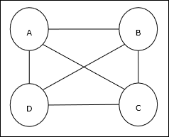
Travelling Salesman Problem (TSP) is a classical optimization problem in which a salesman has to travel n cities, which are connected with each other, keeping the cost as well as the distance travelled minimum. For example, the salesman has to travel a set of 4 cities A, B, C, D and the goal is to find the shortest circular tour, A-B-CD, so as to minimize the cost, which also includes the cost of travelling from the last city D to the first city A.
Matrix Representation
Actually each tour of n-city TSP can be expressed as n × n matrix whose ith row describes the ith citys location. This matrix, M, for 4 cities A, B, C, D can be expressed as follows −
$$M = \begin{bmatrix}A: & 1 & 0 & 0 & 0 \\B: & 0 & 1 & 0 & 0 \\C: & 0 & 0 & 1 & 0 \\D: & 0 & 0 & 0 & 1 \end{bmatrix}$$
Solution by Hopfield Network
While considering the solution of this TSP by Hopfield network, every node in the network corresponds to one element in the matrix.
Energy Function Calculation
To be the optimized solution, the energy function must be minimum. On the basis of the following constraints, we can calculate the energy function as follows −
Constraint-I
First constraint, on the basis of which we will calculate energy function, is that one element must be equal to 1 in each row of matrix M and other elements in each row must equal to 0 because each city can occur in only one position in the TSP tour. This constraint can mathematically be written as follows −
$$\displaystyle\sum\limits_{j=1}^n M_{x,j}\:=\:1\:for \: x\:\in \:\lbrace1,...,n\rbrace$$
Now the energy function to be minimized, based on the above constraint, will contain a term proportional to −
$$\displaystyle\sum\limits_{x=1}^n \left(\begin{array}{c}1\:-\:\displaystyle\sum\limits_{j=1}^n M_{x,j}\end{array}\right)^2$$
Constraint-II
As we know, in TSP one city can occur in any position in the tour hence in each column of matrix M, one element must equal to 1 and other elements must be equal to 0. This constraint can mathematically be written as follows −
$$\displaystyle\sum\limits_{x=1}^n M_{x,j}\:=\:1\:for \: j\:\in \:\lbrace1,...,n\rbrace$$
Now the energy function to be minimized, based on the above constraint, will contain a term proportional to −
$$\displaystyle\sum\limits_{j=1}^n \left(\begin{array}{c}1\:-\:\displaystyle\sum\limits_{x=1}^n M_{x,j}\end{array}\right)^2$$
Cost Function Calculation
Lets suppose a square matrix of (n × n) denoted by C denotes the cost matrix of TSP for n cities where n > 0. Following are some parameters while calculating the cost function −
Cx, y − The element of cost matrix denotes the cost of travelling from city x to y.
Adjacency of the elements of A and B can be shown by the following relation −
$$M_{x,i}\:=\:1\:\: and\:\: M_{y,i\pm 1}\:=\:1$$
As we know, in Matrix the output value of each node can be either 0 or 1, hence for every pair of cities A, B we can add the following terms to the energy function −
$$\displaystyle\sum\limits_{i=1}^n C_{x,y}M_{x,i}(M_{y,i+1}\:+\:M_{y,i-1})$$
On the basis of the above cost function and constraint value, the final energy function E can be given as follows −
$$E\:=\:\frac{1}{2}\displaystyle\sum\limits_{i=1}^n\displaystyle\sum\limits_{x}\displaystyle\sum\limits_{y\neq x}C_{x,y}M_{x,i}(M_{y,i+1}\:+\:M_{y,i-1})\:+$$
$$\:\begin{bmatrix}\gamma_{1} \displaystyle\sum\limits_{x} \left(\begin{array}{c}1\:-\:\displaystyle\sum\limits_{i} M_{x,i}\end{array}\right)^2\:+\: \gamma_{2} \displaystyle\sum\limits_{i} \left(\begin{array}{c}1\:-\:\displaystyle\sum\limits_{x} M_{x,i}\end{array}\right)^2 \end{bmatrix}$$
Here, γ1 and γ2 are two weighing constants.
