Boltzmann Machine

These are stochastic learning processes having recurrent structure and are the basis of the early optimization techniques used in ANN. Boltzmann Machine was invented by Geoffrey Hinton and Terry Sejnowski in 1985. More clarity can be observed in the words of Hinton on Boltzmann Machine.

“A surprising feature of this network is that it uses only locally available information. The change of weight depends only on the behavior of the two units it connects, even though the change optimizes a global measure” - Ackley, Hinton 1985.

Some important points about Boltzmann Machine −

They use recurrent structure.
They consist of stochastic neurons, which have one of the two possible states, either 1 or 0.
Some of the neurons in this are adaptive (free state) and some are clamped (frozen state).
If we apply simulated annealing on discrete Hopfield network, then it would become Boltzmann Machine.

Objective of Boltzmann Machine

The main purpose of Boltzmann Machine is to optimize the solution of a problem. It is the work of Boltzmann Machine to optimize the weights and quantity related to that particular problem.

Architecture

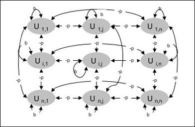
The following diagram shows the architecture of Boltzmann machine. It is clear from the diagram, that it is a two-dimensional array of units. Here, weights on interconnections between units are –p where p > 0. The weights of self-connections are given by b where b > 0.

Training Algorithm

As we know that Boltzmann machines have fixed weights, hence there will be no training algorithm as we do not need to update the weights in the network. However, to test the network we have to set the weights as well as to find the consensus function (CF).

Boltzmann machine has a set of units U_i and U_j and has bi-directional connections on them.

We are considering the fixed weight say w_ij.
w_ij ≠ 0 if U_i and U_j are connected.
There also exists a symmetry in weighted interconnection, i.e. w_ij = w_ji.
w_ii also exists, i.e. there would be the self-connection between units.
For any unit U_i, its state u_i would be either 1 or 0.

The main objective of Boltzmann Machine is to maximize the Consensus Function (CF) which can be given by the following relation

$$CF\:=\:\displaystyle\sum\limits_{i} \displaystyle\sum\limits_{j\leqslant i} w_{ij}u_{i}u_{j}$$

Now, when the state changes from either 1 to 0 or from 0 to 1, then the change in consensus can be given by the following relation −

$$\Delta CF\:=\:(1\:-\:2u_{i})(w_{ij}\:+\:\displaystyle\sum\limits_{j\neq i} u_{i} w_{ij})$$

Here u_i is the current state of U_i.

The variation in coefficient (1 - 2u_i) is given by the following relation −

$$(1\:-\:2u_{i})\:=\:\begin{cases}+1, & U_{i}\:is\:currently\:off\\-1, & U_{i}\:is\:currently\:on\end{cases}$$

Generally, unit U_i does not change its state, but if it does then the information would be residing local to the unit. With that change, there would also be an increase in the consensus of the network.

Probability of the network to accept the change in the state of the unit is given by the following relation −

$$AF(i,T)\:=\:\frac{1}{1\:+\:exp[-\frac{\Delta CF(i)}{T}]}$$

Here, T is the controlling parameter. It will decrease as CF reaches the maximum value.

Testing Algorithm

Step 1 − Initialize the following to start the training −

Weights representing the constraint of the problem
Control Parameter T

Step 2 − Continue steps 3-8, when the stopping condition is not true.

Step 3 − Perform steps 4-7.

Step 4 − Assume that one of the state has changed the weight and choose the integer I, J as random values between 1 and n.

Step 5 − Calculate the change in consensus as follows −

$$\Delta CF\:=\:(1\:-\:2u_{i})(w_{ij}\:+\:\displaystyle\sum\limits_{j\neq i} u_{i} w_{ij})$$

Step 6 − Calculate the probability that this network would accept the change in state

$$AF(i,T)\:=\:\frac{1}{1\:+\:exp[-\frac{\Delta CF(i)}{T}]}$$

Step 7 − Accept or reject this change as follows −

Case I − if R < AF, accept the change.

Case II − if R ≥ AF, reject the change.

Here, R is the random number between 0 and 1.

Step 8 − Reduce the control parameter (temperature) as follows −

T(new) = ⁡0.95T(old)

Step 9 − Test for the stopping conditions which may be as follows −

Temperature reaches a specified value
There is no change in state for a specified number of iterations