- Artificial Neural Network - Home
- Basic Concepts
- Building Blocks
- Learning & Adaptation
- Supervised Learning
- Unsupervised Learning
- Learning Vector Quantization
- Adaptive Resonance Theory
- Kohonen Self-Organizing Feature Maps
- Associate Memory Network
- Hopfield Networks
- Boltzmann Machine
- Brain-State-in-a-Box Network
- Optimization Using Hopfield Network
- Other Optimization Techniques
- Genetic Algorithm
- Applications of Neural Networks
Learning Vector Quantization
Learning Vector Quantization (LVQ), different from Vector quantization (VQ) and Kohonen Self-Organizing Maps (KSOM), basically is a competitive network which uses supervised learning. We may define it as a process of classifying the patterns where each output unit represents a class. As it uses supervised learning, the network will be given a set of training patterns with known classification along with an initial distribution of the output class. After completing the training process, LVQ will classify an input vector by assigning it to the same class as that of the output unit.
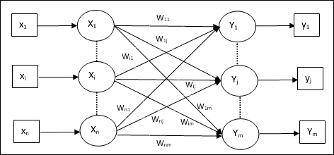
Architecture
Following figure shows the architecture of LVQ which is quite similar to the architecture of KSOM. As we can see, there are n number of input units and m number of output units. The layers are fully interconnected with having weights on them.
Parameters Used
Following are the parameters used in LVQ training process as well as in the flowchart
x = training vector (x1,...,xi,...,xn)
T = class for training vector x
wj = weight vector for jth output unit
Cj = class associated with the jth output unit
Training Algorithm
Step 1 − Initialize reference vectors, which can be done as follows −
Step 1(a) − From the given set of training vectors, take the first m (number of clusters) training vectors and use them as weight vectors. The remaining vectors can be used for training.
Step 1(b) − Assign the initial weight and classification randomly.
Step 1(c) − Apply K-means clustering method.
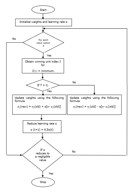
Step 2 − Initialize reference vector $\alpha$
Step 3 − Continue with steps 4-9, if the condition for stopping this algorithm is not met.
Step 4 − Follow steps 5-6 for every training input vector x.
Step 5 − Calculate Square of Euclidean Distance for j = 1 to m and i = 1 to n
$$D(j)\:=\:\displaystyle\sum\limits_{i=1}^n\displaystyle\sum\limits_{j=1}^m (x_{i}\:-\:w_{ij})^2$$
Step 6 − Obtain the winning unit J where D(j) is minimum.
Step 7 − Calculate the new weight of the winning unit by the following relation −
if T = Cj then $w_{j}(new)\:=\:w_{j}(old)\:+\:\alpha[x\:-\:w_{j}(old)]$
if T ≠ Cj then $w_{j}(new)\:=\:w_{j}(old)\:-\:\alpha[x\:-\:w_{j}(old)]$
Step 8 − Reduce the learning rate $\alpha$.
Step 9 − Test for the stopping condition. It may be as follows −
- Maximum number of epochs reached.
- Learning rate reduced to a negligible value.
Flowchart
Variants
Three other variants namely LVQ2, LVQ2.1 and LVQ3 have been developed by Kohonen. Complexity in all these three variants, due to the concept that the winner as well as the runner-up unit will learn, is more than in LVQ.
LVQ2
As discussed, the concept of other variants of LVQ above, the condition of LVQ2 is formed by window. This window will be based on the following parameters −
x − the current input vector
yc − the reference vector closest to x
yr − the other reference vector, which is next closest to x
dc − the distance from x to yc
dr − the distance from x to yr
The input vector x falls in the window, if
$$\frac{d_{c}}{d_{r}}\:>\:1\:-\:\theta\:\:and\:\:\frac{d_{r}}{d_{c}}\:>\:1\:+\:\theta$$
Here, $\theta$ is the number of training samples.
Updating can be done with the following formula −
$y_{c}(t\:+\:1)\:=\:y_{c}(t)\:+\:\alpha(t)[x(t)\:-\:y_{c}(t)]$ (belongs to different class)
$y_{r}(t\:+\:1)\:=\:y_{r}(t)\:+\:\alpha(t)[x(t)\:-\:y_{r}(t)]$ (belongs to same class)
Here $\alpha$ is the learning rate.
LVQ2.1
In LVQ2.1, we will take the two closest vectors namely yc1 and yc2 and the condition for window is as follows −
$$Min\begin{bmatrix}\frac{d_{c1}}{d_{c2}},\frac{d_{c2}}{d_{c1}}\end{bmatrix}\:>\:(1\:-\:\theta)$$
$$Max\begin{bmatrix}\frac{d_{c1}}{d_{c2}},\frac{d_{c2}}{d_{c1}}\end{bmatrix}\:
Updating can be done with the following formula −
$y_{c1}(t\:+\:1)\:=\:y_{c1}(t)\:+\:\alpha(t)[x(t)\:-\:y_{c1}(t)]$ (belongs to different class)
$y_{c2}(t\:+\:1)\:=\:y_{c2}(t)\:+\:\alpha(t)[x(t)\:-\:y_{c2}(t)]$ (belongs to same class)
Here, $\alpha$ is the learning rate.
LVQ3
In LVQ3, we will take the two closest vectors namely yc1 and yc2 and the condition for window is as follows −
$$Min\begin{bmatrix}\frac{d_{c1}}{d_{c2}},\frac{d_{c2}}{d_{c1}}\end{bmatrix}\:>\:(1\:-\:\theta)(1\:+\:\theta)$$
Here $\theta\approx 0.2$
Updating can be done with the following formula −
$y_{c1}(t\:+\:1)\:=\:y_{c1}(t)\:+\:\beta(t)[x(t)\:-\:y_{c1}(t)]$ (belongs to different class)
$y_{c2}(t\:+\:1)\:=\:y_{c2}(t)\:+\:\beta(t)[x(t)\:-\:y_{c2}(t)]$ (belongs to same class)
Here $\beta$ is the multiple of the learning rate $\alpha$ and $\beta\:=\:m \alpha(t)$ for every 0.1 < m < 0.5
