- Artificial Neural Network - Home
- Basic Concepts
- Building Blocks
- Learning & Adaptation
- Supervised Learning
- Unsupervised Learning
- Learning Vector Quantization
- Adaptive Resonance Theory
- Kohonen Self-Organizing Feature Maps
- Associate Memory Network
- Hopfield Networks
- Boltzmann Machine
- Brain-State-in-a-Box Network
- Optimization Using Hopfield Network
- Other Optimization Techniques
- Genetic Algorithm
- Applications of Neural Networks
Neural Network Optimization Techniques
Iterated Gradient Descent Technique
Gradient descent, also known as the steepest descent, is an iterative optimization algorithm to find a local minimum of a function. While minimizing the function, we are concerned with the cost or error to be minimized (Remember Travelling Salesman Problem). It is extensively used in deep learning, which is useful in a wide variety of situations. The point here to be remembered is that we are concerned with local optimization and not global optimization.
Main Working Idea
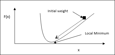
We can understand the main working idea of gradient descent with the help of the following steps −
First, start with an initial guess of the solution.
Then, take the gradient of the function at that point.
Later, repeat the process by stepping the solution in the negative direction of the gradient.
By following the above steps, the algorithm will eventually converge where the gradient is zero.
Mathematical Concept
Suppose we have a function f(x) and we are trying to find the minimum of this function. Following are the steps to find the minimum of f(x).
First, give some initial value $x_{0}\:for\:x$
Now take the gradient $\nabla f$ of function, with the intuition that the gradient will give the slope of the curve at that x and its direction will point to the increase in the function, to find out the best direction to minimize it.
Now change x as follows −
$$x_{n\:+\:1}\:=\:x_{n}\:-\:\theta \nabla f(x_{n})$$
Here, θ > 0 is the training rate (step size) that forces the algorithm to take small jumps.
Estimating Step Size
Actually a wrong step size θ may not reach convergence, hence a careful selection of the same is very important. Following points must have to be remembered while choosing the step size
Do not choose too large step size, otherwise it will have a negative impact, i.e. it will diverge rather than converge.
Do not choose too small step size, otherwise it take a lot of time to converge.
Some options with regards to choosing the step size −
One option is to choose a fixed step size.
Another option is to choose a different step size for every iteration.
Simulated Annealing
The basic concept of Simulated Annealing (SA) is motivated by the annealing in solids. In the process of annealing, if we heat a metal above its melting point and cool it down then the structural properties will depend upon the rate of cooling. We can also say that SA simulates the metallurgy process of annealing.
Use in ANN
SA is a stochastic computational method, inspired by Annealing analogy, for approximating the global optimization of a given function. We can use SA to train feed-forward neural networks.
Algorithm
Step 1 − Generate a random solution.
Step 2 − Calculate its cost using some cost function.
Step 3 − Generate a random neighboring solution.
Step 4 − Calculate the new solution cost by the same cost function.
Step 5 − Compare the cost of a new solution with that of an old solution as follows −
If CostNew Solution < CostOld Solution then move to the new solution.
Step 6 − Test for the stopping condition, which may be the maximum number of iterations reached or get an acceptable solution.
Hopfield Network Technique
Hopfield neural network was invented by Dr. John J. Hopfield in 1982. It consists of a single layer which contains one or more fully connected recurrent neurons. The Hopfield network is commonly used for auto-association and optimization tasks.
Read more: Optimization Using Hopfield Network
