- Artificial Neural Network - Home
- Basic Concepts
- Building Blocks
- Learning & Adaptation
- Supervised Learning
- Unsupervised Learning
- Learning Vector Quantization
- Adaptive Resonance Theory
- Kohonen Self-Organizing Feature Maps
- Associate Memory Network
- Hopfield Networks
- Boltzmann Machine
- Brain-State-in-a-Box Network
- Optimization Using Hopfield Network
- Other Optimization Techniques
- Genetic Algorithm
- Applications of Neural Networks
Kohonen Self-Organizing Feature Maps
Suppose we have some pattern of arbitrary dimensions, however, we need them in one dimension or two dimensions. Then the process of feature mapping would be very useful to convert the wide pattern space into a typical feature space. Now, the question arises why do we require self-organizing feature map? The reason is, along with the capability to convert the arbitrary dimensions into 1-D or 2-D, it must also have the ability to preserve the neighbor topology.
Neighbor Topologies in Kohonen SOM
There can be various topologies, however the following two topologies are used the most −
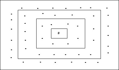
Rectangular Grid Topology
This topology has 24 nodes in the distance-2 grid, 16 nodes in the distance-1 grid, and 8 nodes in the distance-0 grid, which means the difference between each rectangular grid is 8 nodes. The winning unit is indicated by #.
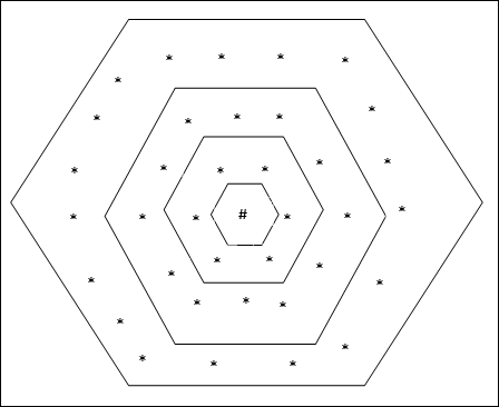
Hexagonal Grid Topology
This topology has 18 nodes in the distance-2 grid, 12 nodes in the distance-1 grid, and 6 nodes in the distance-0 grid, which means the difference between each rectangular grid is 6 nodes. The winning unit is indicated by #.
Architecture
The architecture of KSOM is similar to that of the competitive network. With the help of neighborhood schemes, discussed earlier, the training can take place over the extended region of the network.
Algorithm for training
Step 1 − Initialize the weights, the learning rate α and the neighborhood topological scheme.
Step 2 − Continue step 3-9, when the stopping condition is not true.
Step 3 − Continue step 4-6 for every input vector x.
Step 4 − Calculate Square of Euclidean Distance for j = 1 to m
$$D(j)\:=\:\displaystyle\sum\limits_{i=1}^n \displaystyle\sum\limits_{j=1}^m (x_{i}\:-\:w_{ij})^2$$
Step 5 − Obtain the winning unit J where D(j) is minimum.
Step 6 − Calculate the new weight of the winning unit by the following relation −
$$w_{ij}(new)\:=\:w_{ij}(old)\:+\:\alpha[x_{i}\:-\:w_{ij}(old)]$$
Step 7 − Update the learning rate α by the following relation −
$$\alpha(t\:+\:1)\:=\:0.5\alpha t$$
Step 8 − Reduce the radius of topological scheme.
Step 9 − Check for the stopping condition for the network.
