- Artificial Neural Network - Home
- Basic Concepts
- Building Blocks
- Learning & Adaptation
- Supervised Learning
- Unsupervised Learning
- Learning Vector Quantization
- Adaptive Resonance Theory
- Kohonen Self-Organizing Feature Maps
- Associate Memory Network
- Hopfield Networks
- Boltzmann Machine
- Brain-State-in-a-Box Network
- Optimization Using Hopfield Network
- Other Optimization Techniques
- Genetic Algorithm
- Applications of Neural Networks
Artificial Neural Network - Hopfield Networks
Hopfield neural network was invented by Dr. John J. Hopfield in 1982. It consists of a single layer which contains one or more fully connected recurrent neurons. The Hopfield network is commonly used for auto-association and optimization tasks.
Discrete Hopfield Network
A Hopfield network which operates in a discrete line fashion or in other words, it can be said the input and output patterns are discrete vector, which can be either binary (0,1) or bipolar (+1, -1) in nature. The network has symmetrical weights with no self-connections i.e., wij = wji and wii = 0.
Architecture
Following are some important points to keep in mind about discrete Hopfield network −
This model consists of neurons with one inverting and one non-inverting output.
The output of each neuron should be the input of other neurons but not the input of self.
Weight/connection strength is represented by wij.
Connections can be excitatory as well as inhibitory. It would be excitatory, if the output of the neuron is same as the input, otherwise inhibitory.
Weights should be symmetrical, i.e. wij = wji
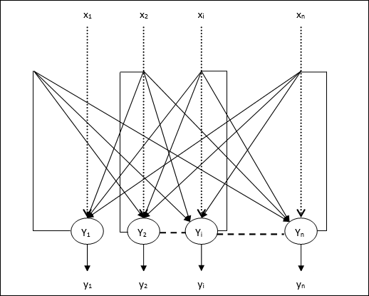
The output from Y1 going to Y2, Yi and Yn have the weights w12, w1i and w1n respectively. Similarly, other arcs have the weights on them.
Training Algorithm
During training of discrete Hopfield network, weights will be updated. As we know that we can have the binary input vectors as well as bipolar input vectors. Hence, in both the cases, weight updates can be done with the following relation
Case 1 − Binary input patterns
For a set of binary patterns s(p), p = 1 to P
Here, s(p) = s1(p), s2(p),..., si(p),..., sn(p)
Weight Matrix is given by
$$w_{ij}\:=\:\sum_{p=1}^P[2s_{i}(p)-\:1][2s_{j}(p)-\:1]\:\:\:\:\:for\:i\:\neq\:j$$
Case 2 − Bipolar input patterns
For a set of binary patterns s(p), p = 1 to P
Here, s(p) = s1(p), s2(p),..., si(p),..., sn(p)
Weight Matrix is given by
$$w_{ij}\:=\:\sum_{p=1}^P[s_{i}(p)][s_{j}(p)]\:\:\:\:\:for\:i\:\neq\:j$$
Testing Algorithm
Step 1 − Initialize the weights, which are obtained from training algorithm by using Hebbian principle.
Step 2 − Perform steps 3-9, if the activations of the network is not consolidated.
Step 3 − For each input vector X, perform steps 4-8.
Step 4 − Make initial activation of the network equal to the external input vector X as follows −
$$y_{i}\:=\:x_{i}\:\:\:for\:i\:=\:1\:to\:n$$
Step 5 − For each unit Yi, perform steps 6-9.
Step 6 − Calculate the net input of the network as follows −
$$y_{ini}\:=\:x_{i}\:+\:\displaystyle\sum\limits_{j}y_{j}w_{ji}$$
Step 7 − Apply the activation as follows over the net input to calculate the output −
$$y_{i}\:=\begin{cases}1 & if\:y_{ini}\:>\:\theta_{i}\\y_{i} & if\:y_{ini}\:=\:\theta_{i}\\0 & if\:y_{ini}\:
Here $\theta_{i}$ is the threshold.
Step 8 − Broadcast this output yi to all other units.
Step 9 − Test the network for conjunction.
Energy Function Evaluation
An energy function is defined as a function that is bonded and non-increasing function of the state of the system.
Energy function Ef, also called Lyapunov function determines the stability of discrete Hopfield network, and is characterized as follows −
$$E_{f}\:=\:-\frac{1}{2}\displaystyle\sum\limits_{i=1}^n\displaystyle\sum\limits_{j=1}^n y_{i}y_{j}w_{ij}\:-\:\displaystyle\sum\limits_{i=1}^n x_{i}y_{i}\:+\:\displaystyle\sum\limits_{i=1}^n \theta_{i}y_{i}$$
Condition − In a stable network, whenever the state of node changes, the above energy function will decrease.
Suppose when node i has changed state from $y_i^{(k)}$ to $y_i^{(k\:+\:1)}$ then the Energy change $\Delta E_{f}$ is given by the following relation
$$\Delta E_{f}\:=\:E_{f}(y_i^{(k+1)})\:-\:E_{f}(y_i^{(k)})$$
$$=\:-\left(\begin{array}{c}\displaystyle\sum\limits_{j=1}^n w_{ij}y_i^{(k)}\:+\:x_{i}\:-\:\theta_{i}\end{array}\right)(y_i^{(k+1)}\:-\:y_i^{(k)})$$
$$=\:-\:(net_{i})\Delta y_{i}$$
Here $\Delta y_{i}\:=\:y_i^{(k\:+\:1)}\:-\:y_i^{(k)}$
The change in energy depends on the fact that only one unit can update its activation at a time.
Continuous Hopfield Network
In comparison with Discrete Hopfield network, continuous network has time as a continuous variable. It is also used in auto association and optimization problems such as travelling salesman problem.
Model − The model or architecture can be build up by adding electrical components such as amplifiers which can map the input voltage to the output voltage over a sigmoid activation function.
Energy Function Evaluation
$$E_f = \frac{1}{2}\displaystyle\sum\limits_{i=1}^n\sum_{\substack{j = 1\\ j \ne i}}^n y_i y_j w_{ij} - \displaystyle\sum\limits_{i=1}^n x_i y_i + \frac{1}{\lambda} \displaystyle\sum\limits_{i=1}^n \sum_{\substack{j = 1\\ j \ne i}}^n w_{ij} g_{ri} \int_{0}^{y_i} a^{-1}(y) dy$$
Here λ is gain parameter and gri input conductance.
