- OBIEE Tutorial
- OBIEE - Home
- OBIEE - Data Warehouse
- OBIEE - Dimensional Modeling
- OBIEE - Schema
- OBIEE - Basics
- OBIEE - Components
- OBIEE - Architecture
- OBIEE - Repositories
- OBIEE - Business Layer
- OBIEE - Presentation Layer
- OBIEE - Testing Repository
- OBIEE - Multiple Logical Table
- OBIEE - Calculation Measures
- OBIEE - Dimension Hierarchies
- OBIEE - Level-Based Measures
- OBIEE - Aggregates
- OBIEE - Variables
- OBIEE - Dashboards
- OBIEE - Filters
- OBIEE - Views
- OBIEE - Prompts
- OBIEE - Security
- OBIEE - Administration
- OBIEE Useful Resources
- OBIEE - Questions Answers
- OBIEE - Quick Guide
- OBIEE - Useful Resources
- OBIEE - Discussion
OBIEE - Quick Guide
OBIEE – Data Warehouse
In today’s competitive market, most successful companies respond quickly to market changes and opportunities. The requirement to respond quickly is by effective and efficient use of data and information. “Data Warehouse” is a central repository of data that is organized by category to support the organization’s decision makers. Once data is stored in a data warehouse, it can be accessed for analysis.
The term "Data Warehouse" was first invented by Bill Inmon in 1990. According to him, “Data warehouse is a subject-oriented, integrated, time-variant and non-volatile collection of data in support of management's decision making process.”
Ralph Kimball provided a definition of data warehouse based on its functionality. He said, “Data warehouse is a copy of transaction data specifically structured for query and analysis.”
Data Warehouse (DW or DWH) is a system used for analysis of data and reporting purposes. They are repositories that saves data from one or more heterogeneous data sources. They store both current and historical data and are used for creating analytical reports. DW can be used to create interactive dashboards for the senior management.
For example, analytic reports can contain data for quarterly comparisons or for annual comparison of sales report for a company.
Data in DW comes from multiple operational systems like sales, human resource, marketing, warehouse management, etc. It contains historical data from different transaction systems but it can also include data from other sources. DW is used to separate data processing and analysis workload from transaction workload and enables to consolidate the data from several data sources.
The Need for Data Warehouse
For example − You have a home loan agency, where data comes from multiple SAP/non-SAP applications such as marketing, sales, ERP, HRM, etc. This data is extracted, transformed and loaded into DW. If you have to do quarterly/annual sales comparison of a product, you cannot use an operational database as this will hang the transaction system. This is where the need for using DW arises.
Characteristics of a Data Warehouse
Some of the key characteristics of DW are −
- It is used for reporting and data analysis.
- It provides a central repository with data integrated from one or more sources.
- It stores current and historical data.
Data Warehouse vs. Transactional System
Following are few differences between Data Warehouse and Operational Database (Transaction System) −
Transactional system is designed for known workloads and transactions like updating a user record, searching a record, etc. However, DW transactions are more complex and present a general form of data.
Transactional system contains the current data of an organization whereas DW normally contains historical data.
Transactional system supports parallel processing of multiple transactions. Concurrency control and recovery mechanisms are required to maintain consistency of the database.
Operational database query allows to read and modify operations (delete and update), while an OLAP query needs only read-only access of stored data (select statement).
DW involves data cleaning, data integration, and data consolidations.
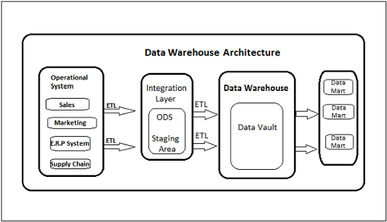
DW has a three-layer architecture − Data Source Layer, Integration Layer, and Presentation Layer. The following diagram shows the common architecture of a Data Warehouse system.
Types of Data Warehouse System
Following are the types of DW system −
- Data Mart
- Online Analytical Processing (OLAP)
- Online Transaction Processing (OLTP)
- Predictive Analysis
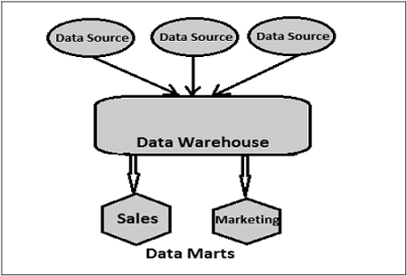
Data Mart
Data Mart is the simplest form of DW and it normally focuses on a single functional area, such as sales, finance or marketing. Hence, data mart usually gets data only from few data sources.
Sources could be an internal transaction system, a central data warehouse, or an external data source application. De-normalization is the norm for data modeling techniques in this system.
Online Analytical Processing (OLAP)
An OLAP system contains less number of transactions but involves complex calculations like use of Aggregations − Sum, Count, Average, etc.
What is Aggregation?
We save tables with aggregated data like yearly (1 row), quarterly (4 rows), monthly (12 rows) and now we want to compare data, like Yearly only 1 row will be processed. However, in an un-aggregated data, all the rows will be processed.
OLAP system normally stores data in multidimensional schemas like Star Schema, Galaxy schemas (with Fact and Dimensional tables are joined in logical manner).
In an OLAP system, response time to execute a query is an effectiveness measure. OLAP applications are widely used by Data Mining techniques to get data from OLAP systems. OLAP databases store aggregated historical data in multi-dimensional schemas. OLAP systems have data latency of a few hours as compared to Data Marts where latency is normally closer to few days.
Online Transaction Processing (OLTP)
An OLTP system is known for large number of short online transactions like insert, update, delete, etc. OLTP systems provide fast query processing and also responsible to provide data integrity in multi-access environment.
For an OLTP systems, effectiveness is measured by the number of transactions processed per second. OLTP systems normally contain only current data. The schema used to store transactional databases is the entity model. Normalization is used for data modeling techniques in OLTP system.
OLTP vs OLAP
The following illustration shows the key differences between an OLTP and OLAP system.
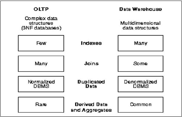
Indexes − In an OLTP system, there are only few indexes while in an OLAP system there are many indexes for performance optimization.
Joins − In an OLTP system, large number of joins and data is normalized; however, in an OLAP system there are less joins and de-normalized.
Aggregation − In an OLTP system, data is not aggregated while in an OLAP database more aggregations are used.
OBIEE – Dimensional Modeling
Dimensional modeling provides set of methods and concepts that are used in DW design. According to DW consultant, Ralph Kimball, dimensional modeling is a design technique for databases intended to support end-user queries in a data warehouse. It is oriented around understandability and performance. According to him, although transaction-oriented ER is very useful for the transaction capture, it should be avoided for end-user delivery.
Dimensional modeling always uses facts and dimension tables. Facts are numerical values which can be aggregated and analyzed on the fact values. Dimensions define hierarchies and description on fact values.
Dimension Table
Dimension table stores the attributes that describe objects in a Fact table. A Dimension table has a primary key that uniquely identifies each dimension row. This key is used to associate the Dimension table to a Fact table.
Dimension tables are normally de-normalized as they are not created to execute transactions and only used to analyze data in detail.
Example
In the following dimension table, the customer dimension normally includes the name of customers, address, customer id, gender, income group, education levels, etc.
| Customer ID | Name | Gender | Income | Education | Religion |
|---|---|---|---|---|---|
| 1 | Brian Edge | M | 2 | 3 | 4 |
| 2 | Fred Smith | M | 3 | 5 | 1 |
| 3 | Sally Jones | F | 1 | 7 | 3 |
Fact Tables
Fact table contains numeric values that are known as measurements. A Fact table has two types of columns − facts and foreign key to dimension tables.
Measures in Fact table are of three types −
Additive − Measures that can be added across any dimension.
Non-Additive − Measures that cannot be added across any dimension.
Semi-Additive − Measures that can be added across some dimensions.
Example
| Time ID | Product ID | Customer ID | Unit Sold |
|---|---|---|---|
| 4 | 17 | 2 | 1 |
| 8 | 21 | 3 | 2 |
| 8 | 4 | 1 | 1 |
This fact tables contains foreign keys for time dimension, product dimension, customer dimension and measurement value unit sold.
Suppose a company sells products to customers. Every sale is a fact that happens within the company, and the fact table is used to record these facts.
Common facts are − number of unit sold, margin, sales revenue, etc. The dimension table list factors like customer, time, product, etc. by which we want to analyze the data.
Now if we consider the above Fact table and Customer dimension then there will also be a Product and time dimension. Given this fact table and these three dimension tables, we can ask questions like: How many watches were sold to male customers in 2010?
Difference between Dimension and Fact Table
The functional difference between dimension tables and fact tables is that fact tables hold the data we want to analyze and dimension tables hold the information required to allow us to query it.
Aggregate Table
Aggregate table contains aggregated data which can be calculated by using different aggregate functions.
An aggregate function is a function where the values of multiple rows are grouped together as input on certain criteria to form a single value of more significant meaning or measurement.
Common aggregate functions include −
- Average()
- Count()
- Maximum()
- Median()
- Minimum()
- Mode()
- Sum()
These aggregate tables are used for performance optimization to run complex queries in a data warehouse.
Example
You save tables with aggregated data like yearly (1 row), quarterly (4 rows), monthly (12 rows) and now you have to do comparison of data, like Yearly only 1 row will be processed. However in an un-aggregated table, all the rows will be processed.
| MIN | Returns the smallest value in a given column |
| MAX | Returns the largest value in a given column |
| SUM | Returns the sum of the numeric values in a given column |
| AVG | Returns the average value of a given column |
| COUNT | Returns the total number of values in a given column |
| COUNT (*) | Returns the number of rows in a table |
Select Avg (salary) from employee where title = ‘developer’. This statement will return the average salary for all employees whose title is equal to 'Developer'.
Aggregations can be applied at database level. You can create aggregates and save them in aggregate tables in the database or you can apply aggregate on the fly at the report level.
Note − If you save aggregates at the database level it saves time and provides performance optimization.
OBIEE – Schema
Schema is a logical description of the entire database. It includes the name and description of records of all types including all associated data-items and aggregates. Much like a database, DW also requires to maintain a schema. Database uses relational model, while DW uses Star, Snowflake, and Fact Constellation schema (Galaxy schema).
Star Schema
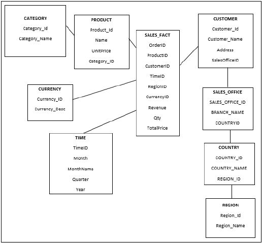
In a Star Schema, there are multiple dimension tables in de-normalized form that are joined to only one fact table. These tables are joined in a logical manner to meet some business requirement for analysis purpose. These schemas are multidimensional structures which are used to create reports using BI reporting tools.
Dimensions in Star schemas contain a set of attributes and Fact tables contain foreign keys for all dimensions and measurement values.
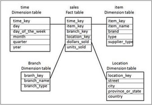
In the above Star Schema, there is a fact table “Sales Fact” at the center and is joined to 4 dimension tables using primary keys. Dimension tables are not further normalized and this joining of tables is known as Star Schema in DW.
Fact table also contains measure values − dollar_sold and units_sold.
Snowflakes Schema
In a Snowflakes Schema, there are multiple dimension tables in normalized form that are joined to only one fact table. These tables are joined in a logical manner to meet some business requirement for analysis purpose.
Only difference between a Star and Snowflakes schema is that dimension tables are further normalized. The normalization splits up the data into additional tables. Due to normalization in the Snowflake schema, the data redundancy is reduced without losing any information and therefore it becomes easy to maintain and saves storage space.
In above Snowflakes Schema example, Product and Customer table are further normalized to save storage space. Sometimes, it also provides performance optimization when you execute a query that requires processing of rows directly in normalized table so it doesn’t process rows in primary Dimension table and comes directly to Normalized table in Schema.
Granularity
Granularity in a table represents the level of information stored in the table. High granularity of data means that data is at or near the transaction level, which has more detail. Low granularity means that data has low level of information.
A fact table is usually designed at a low level of granularity. This means that we need to find the lowest level of information that can be stored in a fact table. In date dimension, the granularity level could be year, month, quarter, period, week, and day.
The process of defining granularity consists of two steps −
- Determining the dimensions that are to be included.
- Determining the location to place the hierarchy of each dimension of information.
Slowly Changing Dimensions
Slowly changing dimensions refer to changing value of an attribute over time. It is one of the common concepts in DW.
Example
Andy is an employee of XYZ Inc. He was first located in New York City in July 2015. Original entry in the employee lookup table has the following record −
| Employee ID | 10001 |
|---|---|
| Name | Andy |
| Location | New York |
At a later date, he has relocated to LA, California. How should XYZ Inc. now modify its employee table to reflect this change?
This is known as "Slowly Changing Dimension" concept.
There are three ways to solve this type of problem −
Solution 1
The new record replaces the original record. No trace of the old record exists.
Slowly Changing Dimension, the new information simply overwrites the original information. In other words, no history is kept.
| Employee ID | 10001 |
|---|---|
| Name | Andy |
| Location | LA, California |
Benefit − This is the easiest way to handle the Slowly Changing Dimension problem as there is no need to keep track of the old information.
Disadvantage − All historical information is lost.
Use − Solution 1 should be used when it is not required for DW to keep track of historical information.
Solution 2
A new record is entered into the Employee dimension table. So the employee, Andy, is treated as two people.
A new record is added to the table to represent the new information and both the original and new record will be present. The new record gets its own primary key as follows −
| Employee ID | 10001 | 10002 |
|---|---|---|
| Name | Andy | Andy |
| Location | New York | LA, California |
Benefit − This method allows us to store all the historical information.
Disadvantage − Size of the table grows faster. When the number of rows for the table is very high, space and performance of table can be a concern.
Use − Solution 2 should be used when it is necessary for DW to keep historical data.
Solution 3
The original record in Employee dimension is modified to reflect the change.
There will be two columns to indicate the particular attribute, one indicates original value and other indicates the new value. There will also be a column that indicates when the current value becomes active.
| Employee ID | Name | Original Location | New Location | Date Moved |
|---|---|---|---|---|
| 10001 | Andy | New York | LA, California | July 2015 |
Benefits − This does not increase the size of the table, since new information is updated. This allows us to keep historical information.
Disadvantage − This method doesn’t keep all history when an attribute value is changed more than once.
Use − Solution 3 should only be used when it is required for DW to keep information of historical changes.
Normalization
Normalization is the process of decomposing a table into less redundant smaller tables without losing any information. So Database normalization is the process of organizing the attributes and tables of a database to minimize data redundancy (duplicate data).
Purpose of Normalization
It is used to eliminate certain types of data (redundancy/ replication) to improve consistency.
It provides maximum flexibility to meet future information needs by keeping tables corresponding to object types in their simplified forms.
It produces a clearer and readable data model.
Advantages
- Data integrity.
- Enhances data consistency.
- Reduces data redundancy and space required.
- Reduces update cost.
- Maximum flexibility in responding to ad-hoc queries.
- Reduces the total number of rows per block.
Disadvantages
Slow performance of queries in database because joins have to be performed to retrieve relevant data from several normalized tables.
You have to understand the data model in order to perform proper joins among several tables.
Example
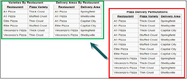
In the above example, the table inside the green block represents a normalized table of the one inside the red block. The table in green block is less redundant and also with less number of rows without losing any information.
OBIEE – Basics
OBIEE stands for Oracle Business Intelligence Enterprise Edition, a set of Business Intelligence tools and is provided by Oracle Corporation. It enables the user to deliver robust set of reporting, ad-hoc query and analysis, OLAP, dashboard, and scorecard functionality with a rich end-user experience that includes visualization, collaboration, alerts and many more options.
Key Points
OBIEE provides robust reporting which makes data easier for business users to access.
OBIEE provides a common infrastructure for producing and delivering enterprise reports, scorecards, dashboards, ad-hoc analysis, and OLAP analysis.
OBIEE reduces cost with a proven web-based service-oriented architecture that integrates with existing IT infrastructure.
OBIEE enables the user to include rich visualization, interactive dashboards, a vast range of animated charting options, OLAP-style interactions, innovative search, and actionable collaboration capabilities to increase the user adoption. These capabilities enable your organization to make better decisions, take informed actions, and implement more-efficient business processes.
Competitors in the Market
The main competitors of OBIEE are Microsoft BI tools, SAP AG Business Objects, IBM Cognos and SAS Institute Inc.
As OBIEE enables the user to create interactive dashboards, robust reports, animated charts and also because of its cost-effectiveness, it is widely used by many companies as one of main tool for Business Intelligence solution.
Advantages of OBIEE
OBIEE provides various types of visualizations to insert in dashboards to make it more interactive. It allows you to create flash reports, report templates, and ad-hoc reporting for end users. It provides close integration with major data sources and can also be integrated with third party vendors like Microsoft to embed data in PowerPoint presentations and word documents.
Following are the key features and benefits of OBIEE tool −
| Features | Key Benefits of OBIEE |
|---|---|
| Interactive Dashboards | Provides fully interactive dashboards and reports with a rich variety of visualizations |
| Self-serve Interactive Reporting | Enable business users to create new analyses from scratch or modify existing analyses without any help from IT |
| Enterprise Reporting | Allows the creation of highly formatted templates, reports, and documents such as flash reports, checks, and more |
| Proactive Detection and Alerts | provides a powerful, near-real-time, multi-step alert engine that can trigger workflows based on business events and notify stakeholders via their preffered medium and channel |
| Actionable Intelligence | Turns insights into actions by providing the ability to invoke business processes from within the business intelligence dashboards and reports |
| Microsoft Office Integration | Enables users to embed up-to-the-minute corporate data in Microsoft PowerPoint, word, and Excel documents |
| Spatial Intelligence via Map-based Visualizations | Allows users to visualize their analytics data using maps, bringing the intuitiveness of spatial visualization to the world of business intelligence |
How to Sign in to OBIEE?
To sign into OBIEE, you can use web URL, user name and password.
To sign into Oracle BI Enterprise Edition −
Step 1 − In the Web browser address bar, enter URL to access OBIEE.
The "Sign In page" is displayed.
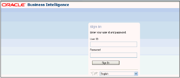
Step 2 − Enter your user name and password → Select the language (You can change the language by selecting another language in the User Interface Language field in the My Account dialog Preferences tab") → Click on Sign In tab.
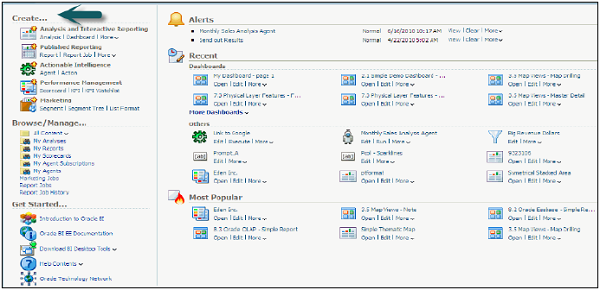
It will take you to the next page as per configuration: OBIEE homepage as shown in the following image or to My Dashboard page/Personal Dashboard or a Dashboard specific to your job role.
OBIEE – Components
OBIEE components are mainly divided into two types of components −
- Server Components
- Client Components
Server components are responsible to run OBIEE system and client components interact with user to create reports and dashboards.
Server Components
Following are the server components −
- Oracle BI (OBIEE) Server
- Oracle Presentation Server
- Application Server
- Scheduler
- Cluster Controller
Oracle BI Server
This component is the heart of OBIEE system and is responsible to communicate with other components. It generates queries for report request and they are sent to database for execution.
It is also responsible for managing repository components which are presented to the user for report generation, handles security mechanism, multi user environment, etc.
OBIEE Presentation Server
It takes the request from users via browser and passes all requests to OBIEE server.
OBIEE Application Server
OBIEE Application Server helps to work on client components and Oracle provides Oracle10g Application server with OBIEE suite.
OBIEE Scheduler
It is responsible to schedule jobs in OBIEE repository. When you create a repository, OBIEE also create a table inside the repository which saves all schedule-related information. This component is also mandatory to run agents in 11g.
All jobs which are scheduled by the Scheduler can be monitored by the job manager.
Client Components
Following are some client components −
Web-based OBIEE Client
Following tools are provided in OBIEE web-based client −
- Interactive Dashboards
- Oracle Delivers
- BI Publisher
- BI Presentation Service Administrator
- Answers
- Disconnected Analytics
- MS Office Plugin
Non-Web based Client
In Non-Web based client, following are the key components −
OBIEE Administration − It is used to build repositories and has three layers − Physical, Business, and Presentation.
ODBC Client − It is used to connect to database and execute SQL commands.
OBIEE – Architecture
OBIEE Architecture involves various BI system components which are required to process the end user’s request.
How OBIEE System Actually Works?
The initial request from the end user is sent to the Presentation server. The Presentation server converts this request in logical SQL and forwards it to BI server component. BI server converts this into physical SQL and sends it to database to get the required result. This result is presented to the end user through the same way.
The following diagram shows detailed OBIEE Architecture −
OBIEE Architecture contains Java and non-Java components. Java components are Web Logic Server components and non-Java components are called Oracle BI system component.
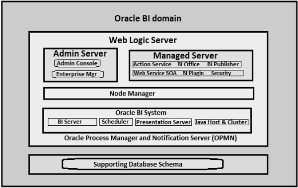
Web Logic Server
This part of OBIEE system contains Admin Server and Managed Server. Admin server is responsible for managing the start and stop processes for Managed server. Managed Server comprises of BI Plugin, Security, Publisher, SOA, BI Office, etc.
Node Manager
Node Manager triggers the auto start, stop, restart activities and provides process management activities for Admin and Managed server.
Oracle Process Manager and Notification Server (OPMN)
OPMN is used to start and stop all components of BI system. It is managed and controlled by Fusion Middleware Controller.
Oracle BI System Components
These are non-Java components in an OBIEE system.
Oracle BI Server
This is the heart of Oracle BI system and is responsible for providing data and query access capabilities.
BI Presentation Server
It is responsible to present data from BI server to web clients which is requested by the end users.
Scheduler
This component provides scheduling capability in BI system and it has its own scheduler to schedule jobs in OBIEE system.
Oracle BI Java Host
This is responsible for enabling BI Presentation server to support various Java tasks for BI Scheduler, Publisher and graphs.
BI Cluster Controller
This is used for load balancing purposes to ensure that the load is evenly assigned to all BI server processes.
OBIEE – Repositories
OBIEE repository contains all metadata of the BI Server and is managed through the administration tool. It is used to store information about the application environment such as −
- Data Modeling
- Aggregate Navigation
- Caching
- Security
- Connectivity Information
- SQL Information
The BI Server can access multiple repositories. OBIEE Repository can be accessed using the following path −
BI_ORACLE_HOME/server/Repository -> Oracle 10g
ORACLE_INSTANCE/bifoundation/OracleBIServerComponent/coreapplication_obisn/-> Oracle 11g
OBIEE repository database is also known as a RPD because of its file extension. The RPD file is password protected and you can only open or create RPD files using Oracle BI Administration tool. To deploy an OBIEE application, the RPD file must be uploaded to Oracle Enterprise Manager. After uploading the RPD, the RPD password then must be entered into Enterprise Manager.
Designing an OBIEE Repository using Administration Tool
It is a three layer process − starting from Physical Layer (Schema Design), Business Model Layer, Presentation Layer.
Creating the Physical Layer
Following are the common steps involved in creating the Physical Layer −
- Create physical joins between the Dimension and Fact tables.
- Change the names in the physical layer if required.
The physical layer of repository contains information about the data sources. To create the schema in the physical layer you need to import metadata from databases and other data sources.
Note − Physical layer in OBIEE supports multiple data sources in a single repository - i.e. data sets from 2 different data sources can be performed in OBIEE.
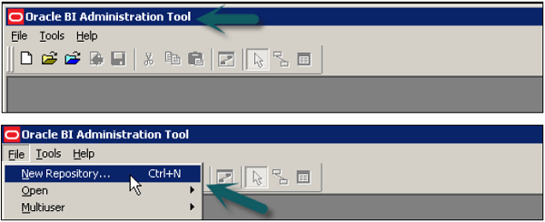
Create a New Repository
Go to Start → Programs → Oracle Business Intelligence → BI Administration → Administration Tool → File → New Repository.
A new window will open → Enter the name of Repository → Location (It tells the default location of Repository directory) → to import metadata select radio button → Enter Password → Click Next.
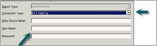
Select the connection type → Enter Data Source name and User name and password to connect to data source → Click Next.
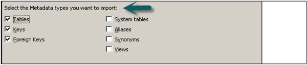
Accept the meta types you want to import → You can select Tables, Keys, Foreign Keys, System tables, Synonyms, Alias, Views, etc. → Click Next.
Once you click Next, you will see Data Source view and Repository view. Expand the Schema name and select tables you want to add to Repository using Import Selected button → Click Next.
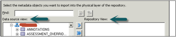
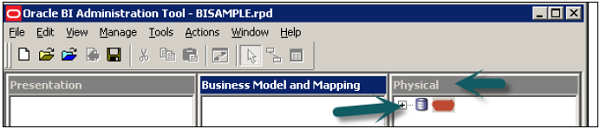
Connection Pool window opens up → Click OK → Importing window → Finish to open the repository as shown in the following image.
Expand the Data Source → Schema name to see the list of tables Imported in Physical Layer in the new Repository.
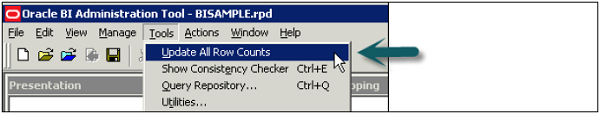
Verify Connection and Number of Rows in Tables Under Physical Layer
Go to tools → Update all rows counts → Once it is completed you can move the cursor on the table and also for individual columns. To see Data of a table, right-click on Table name → View Data.
Create Alias in Repository
It is advisable that you use table aliases frequently in the Physical layer to eliminate extra joins. Right-click on table name and select New Object → Alias.
Once you create an Alias of a table it shows up under the same Physical Layer in the Repository.
Create Primary Keys and Joins in Repository Design
Physical Joins
When you create a repository in OBIEE system, physical join is commonly used in the Physical layer. Physical joins help to understand how two tables should be joined to each other. Physical joins are normally expressed with the use of Equal operator.
You can also use a physical join in BMM layer, however, it is very rarely seen. The purpose of using a physical join in BMM layer is to override the physical join in the physical layer. It allows users to define more complex joining logic as compared to physical join in the physical layer so it works similar to complex join in the physical layer. Therefore, if we are using a complex join in the physical layer for applying more join conditions, there is no need to use a physical join in BMM layer again.
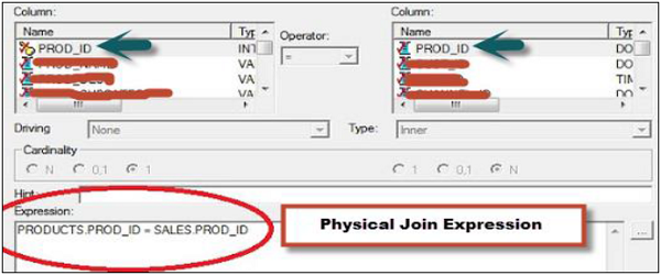
In the above snapshot, you can see a physical join between two table names − Products and Sales. Physical Join expression tells how the tables should be joined with each other as shown in the snapshot.
It is always recommended to use a physical join in the physical layer and complex join in BMM layer as much as possible to keep Repository design simple. Only when there is an actual need for a different join, then use a physical join in BMM layer.
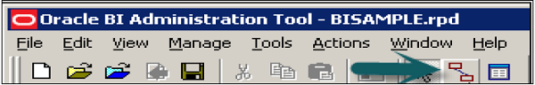
Now to join tables while designing Repository, select all the tables in the Physical layer → Right-click → Physical diagram → Selected objects only option or you can also use Physical Diagram button at the top.
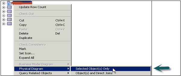
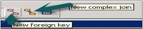
Physical Diagram box as shown in the following image appears with all the table names added. Select the new foreign key at the top and select Dim and Fact table to join.
Foreign Key in Physical Layer
A Foreign key in the physical layer is used to define Primary key-Foreign key relation between two tables. When you create it in the physical diagram, you have to point first the dimension and then the fact table.
Note − When you import tables from schema into RPD Physical Layer, you can also select KEY and FOREIGN KEY along with the table data, then the primary key-foreign key joins are automatically defined, however it is not recommended from performance point of view.
The table you click first, it creates one-to-one or one-to-many relationship that joins column in first table with foreign key column in the second table → Click Ok. The join will be visible in Physical Diagram box between two tables. Once tables are joined, close the Physical diagram box using ‘X’ option.
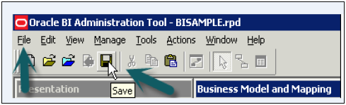
To save the new Repository go to File → Save or click the save button at the top.
Creating Business Model and Mapping Layer of a Repository
It defines the business or logical model of objects and their mapping between business model and Schema in the physical layer. It simplifies the Physical Schema and maps the user business requirement to physical tables.
The Business Model and Mapping layer of OBIEE system administration tool can contain one or more business model objects. A business model object defines the business model definitions and the mappings from logical to physical tables for the business model.
Following are the steps to build the Business Model and Mapping layer of a repository −
- Create a business model
- Examine logical joins
- Examine logical columns
- Examine logical table sources
- Rename logical table objects manually
- Rename logical table objects using the rename wizard and deleting unnecessary logical objects
- Creating measures (Aggregations)
Create a Business Model
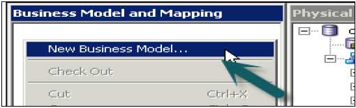
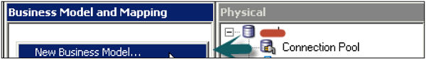
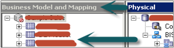
Right-click on Business Model and Mapping Space → New Business Model.
Enter the name of Business Model → click OK.
In the physical layer, select all the tables/alias tables to be added to Business Model and drag to Business Model. You can also add tables one by one. If you drag all the tables simultaneously, it will keep keys and joins between them.
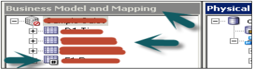
Also note the difference in icon of Dimension and Fact tables. Last table is Fact table and top 3 are dimension tables.
Now right-click on Business model → select Business Model diagram → Whole diagram → All tables are dragged simultaneously so it will keep all joins and keys. Now double click on any join to open the logical join box.
Logical and Complex Joins in BMM
Joins in this layer are logical joins. It doesn’t show expressions and tells the type of join between tables. It helps Oracle BI server to understand the relationships between the various pieces of the business model. When you send a query to Oracle BI server, the server determines how to construct physical queries by examining how the logical model is structured.
Click Ok → Click ‘X’ to close the Business model diagram.
To examine logical columns and logical table sources, first expand the columns under tables in BMM. Logical columns were created for each table when you dragged all tables from the physical layer. To check logical table sources → Expand the source folder under each table and it points to the table in the physical layer.
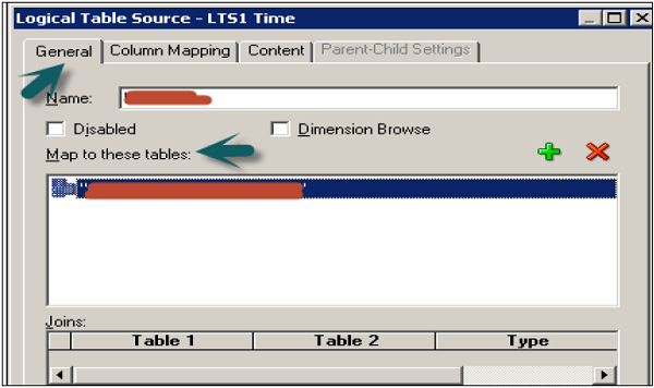
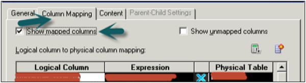
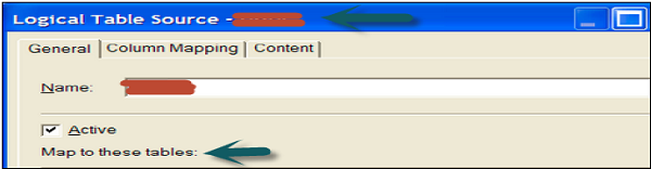
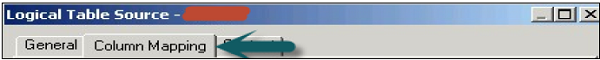
Double-click the logical table source (not the logical table) to open the logical table source dialog box → General tab → rename the logical table source. Logical table to physical table mapping is defined under "Map to these tables" option.
Next, Column mapping tab defines the logical column to physical column mappings. If mappings are not shown, check the option → Show mapped columns.
Complex Joins
There is no specific explicit complex join like in OBIEE 11g. It only exists in Oracle 10g.
Go to Manage → Joins → Actions → New → Complex Join.
When complex joins are used in the BMM layer, they act as placeholders. They allow the OBI Server to decide on which are the best joins between fact and dimension logical table source to satisfy the request.
Rename Logical Objects Manually
To rename logical table objects manually, click the column name under the Logical table in BMM. You can also right-click on column name and select option rename, to rename the object.
This is known as manual method to rename objects.
Rename Objects Using the Rename Wizard
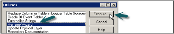
Go to Tools → Utilities → Rename Wizard → Execute to open the rename wizard.
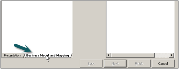
In the Select Objects screen, click Business Model and Mapping. It will show Business Model name → Expand Business Model name → Expand logical tables.
Select all the columns under the logical table to rename using the Shift key → Click Add. Similarly, add columns from all other logical Dim and Fact tables → click Next.
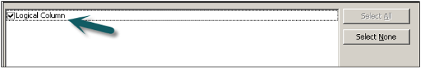
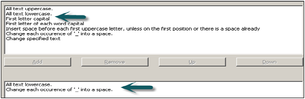
It shows all logical columns/tables added to wizard → Click Next to open Rules screen → Add rules from the list to rename like : A;; text lower case and change each occurrence of ‘_’ to space as shown in the following snapshot.
Click Next → finish. Now, if you expand Object names under logical tables in Business model and Objects in the physical layer, objects under BMM are renamed as required.
Delete Unnecessary Logical Objects
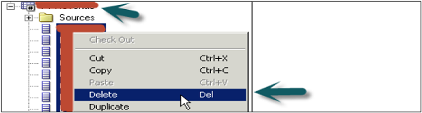
In the BMM layer, expand Logical tables → select objects to be deleted → right-click → Delete → Yes.
Create Measures (Aggregations)
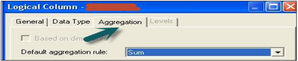
Double-click on the column name in the logical Fact table → Go to Aggregation tab and select the Aggregate function from the dropdown list → Click OK.
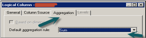
Measures represent data that is additive, such as total revenue or total quantity. Click on save option at top to save the repository.
Creating the Presentation Layer of a Repository
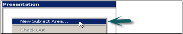
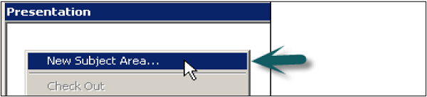
Right-click on Presentation area → New Subject Area → In the General tab enter the name of subject area (Recommended similar to Business Model) → Click OK.
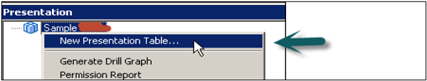
Once subject area is created, right click on subject area → New presentation table → Enter the name of the presentation table → Click OK (Add number of presentation tables equal to number of parameters required in the report).
Now, to create columns under Presentation tables → Select the objects under logical tables in BMM and drag them to Presentation tables under subject area (Use Ctrl key to select multiple objects for dragging). Repeat the process and add the logical columns to the remaining presentation tables.
Rename and Reorder Objects in Presentation Layer
You can rename the objects in Presentation tables by a double-click on logical objects under subject area.
In General tab → Deselect the check box Use Logical column name → Edit the name field → Click OK.

Similarly, you can rename all the objects in the Presentation layer without changing their name in BMM layer.
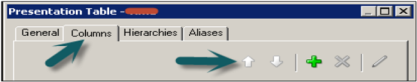
To order the columns in a table, double-click on the table name under Presentation → Columns → Use up and down arrows to change the order → Click OK.
Similarly, you can change objects order in all presentation tables under Presentation area. Go to File → Click Save to save the Repository.
Check Consistency and Load the Repository for Query Analysis
Go to File → Check Global Consistency → You will receive the following message → Click Yes.
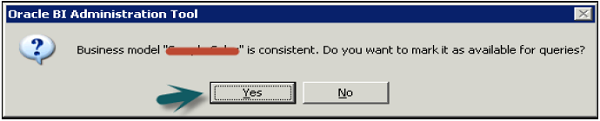
Once you click OK → Business model under BMM will change to Green → Click save the repository without checking global consistency again.
Disable Caching
To improve query performance, it is advised to disable BI server cache option.
Open a browser and enter the following URL to open Fusion Middleware Control Enterprise Manager: http://<machine name>:7001/em
Enter the user name and password and click Login.
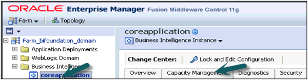
On the left side, expand Business Intelligence → coreapplication → Capacity Management tab → Performance.
Enable BI Server Cache section is by default checked → Click Lock and Edit Configuration → Click Close.
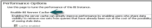
Now deselect cache enabled option → It is used to improve query performance → Apply → Activate Changes → Completed Successfully.
Loading the Repository
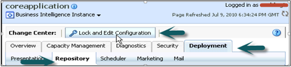
Go to Deployment tab → Repository → Lock and Edit Configuration → Completed Successfully.
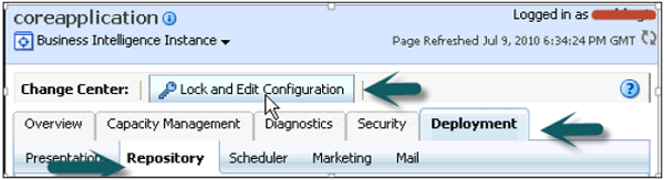
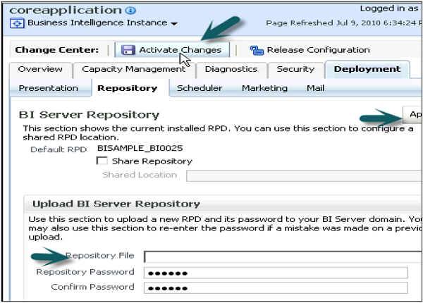
Click Upload BI Server Repository section → Browse to open the Choose file dialog box → Select the Repository .rpd file and click on Open → Enter Repository password → Apply → Activate Changes.
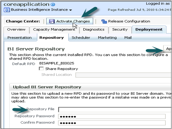
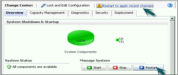
Activate Changes → Completed Successfully → Click Restart to apply recent changes option on top of the screen → Click Yes.

Repository is successfully created and loaded for query Analysis.
OBIEE – Business Layer
Business Layer defines the business or logical model of objects and their mapping between business model and Schema in the physical layer. It simplifies the Physical Schema and maps the user business requirement to physical tables.
The business model and mapping layer of OBIEE system administration tool can contain one or more business model objects. A business model object defines the business model definitions and the mappings from logical to physical tables for the business model.
The business model is used to simplify the schema structure and maps the users’ business requirement to physical data source. It involves creation of logical tables and columns in the business model. Each logical table can have one or more physical objects as sources.
There are two categories of logical tables − fact and dimension. Logical fact tables contain the measures on which analysis is done and Logical dimension tables contain the information about measures and objects in Schema.
While creating a new repository using OBIEE administration tool, once you define the physical layer, create joins and identify foreign keys. The next step is to create a business model and mapping BMM layer of the repository.
Steps involved in defining Business Layer −
- Create a business model
- Examine logical joins
- Examine logical columns
- Examine logical table sources
- Rename logical table objects manually
- Rename logical table objects using the rename wizard and delete unnecessary logical object
- Creating measures (Aggregations)
Create Business Layer in the Repository
To create a business layer in the repository, right-click → New Business Model → Enter the name of Business Model and click OK. You can also add description of this Business Model if you want.

Logical Tables and Objects in BMM Layer
Logical tables in OBIEE repository exist in the Business Model and Mapping BMM layer. The business model diagram should contain at least two logical tables and you need to define relationships between them.
Each logical table should have one or more logical columns and one or more logical table sources associated with it. You can also change the logical table name, reorder the objects in logical table and define logical joins using primary and foreign keys.
Create Logical Tables Under BMM Layer
There are two ways of creating logical tables/objects in BMM layer −
First method is dragging physical tables to Business Model which is the fastest way of defining logical tables. When you drag the tables from the physical layer to BMM layer, it also preserves the joins and keys automatically. If you want you can change the joins and keys in logical tables, it doesn’t affect objects in the physical layer.
Select physical tables/alias tables under the physical layer that you want to add to Business Model Layer and drag those table under BMM layer.
These tables are known as logical tables and columns are called Logical objects in Business Model and Mapping Layer.
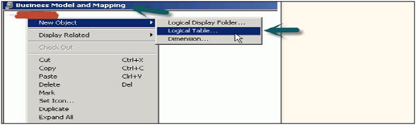
Second method is to create a logical table manually. In the Business Model and Mapping layer, right-click the business model → Select New Object → Logical Table → Logical Table dialog box appears.
Go to General tab → Enter name for the logical table → Type a description of the table → Click OK.
Create Logical Columns
Logical columns in BMM layer are automatically created when you drag tables from the physical layer to the business model layer.
If the logical column is a primary key, this column is displayed with the key icon. If the column has an aggregation function, it is displayed with a sigma icon. You can also reorder logical columns in the Business Model and Mapping layer.
Create a Logical Column
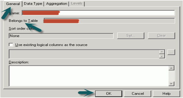
In BMM layer, right-click on logical table → select New Object → Logical Column → Logical Column dialog box will appear, click General tab.
Type a name for the logical column. The name of the business model and the logical table appear in the “Belongs to Table” field just below column name → click OK.
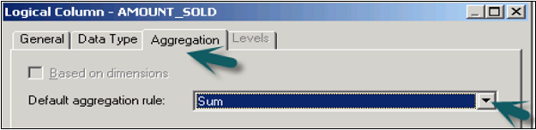
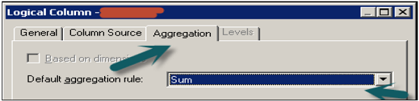
You can also apply Aggregations on the logical columns. Click Aggregation tab → Select Aggregation rule from the dropdown list → Click OK.
Once you apply Aggregate function on a column, logical column icon is changed to show Aggregation rule is applied.
You can also move or copy logical column in tables −
In the BMM layer, you can select multiple columns to move. In the Sources for moved columns dialog box, in the Action area, select an action. If you select Ignore, no logical source will be added in the Sources folder of the table.
If you click on Create new, a copy of the logical source with the logical column will be created in the Sources folder. If you select Use existing option, from the drop-down list, you must select a logical source from the Sources folder of the table.
Create Logical Complex Joins / Logical Foreign Keys
Logical tables in BMM layer are joined to each other using logical joins. Cardinality is one of the key defining parameter in logical joins. Cardinality relation one-to-many means that each row in first logical dimension table there are 0, 1, many rows in second logical table.
Conditions to Create Logical Joins Automatically
When you drag all the tables of the physical layer to business model layer, logical joins are automatically created in Repository. This condition rarely happens only in case of simple business models.
When logical joins are same as physical joins, they are automatically created. Logical joins in BMM layer are created in two ways −
- Business Model Diagram (already covered while designing repository)
- Joins Manager
Logical joins in BMM layer cannot be specified using expressions or columns on which to create the join like in the physical layer where expressions and column names are shown on which physical joins are defined.
Create Logical Joins/Logical Foreign keys Using Join Manager Tool
First let us see how to create logical foreign keys using Join Manager.
In the Administration Tool toolbar, go to Manage → Joins. The Joins Manager dialog box appears → Go to Action tab → New → Logical Foreign Key.
Now in the Browse dialog box, double-click a table → The Logical Foreign Key dialog box appears → Enter the name for the foreign key → From Table drop-down list of the dialog box, select the table that the foreign key references → Select the columns in the left table that the foreign key references → Select the columns in the right table that make up the foreign key columns → Select the join type from the Type drop-down list. To open the Expression Builder, click the button to the right of the Expression pane → The expression displays in the Expression pane → click OK to save the work.
Create a Logical Complex Join using Join Manager
Logical complex joins are recommended in Business Model and mapping layer as compared to the use of logical foreign keys.
In the Administration Tool toolbar, go to Manage → Join → Joins Manager dialog box appears → Go to Action → Click New → Logical Complex Join.
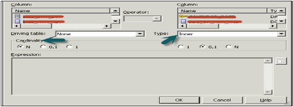
It will open a logical Join dialog box → Type a name for the complex join → In the table drop-down lists on the left and right side of the dialog box, select the tables that the complex join references → Select the join type from the Type drop-down list → Click OK.
Note − You can also define a table as driving table from the drop-down list. This is used for performance optimization when the table size is too large. If the table size is small, less than 1000 rows, it shouldn’t be defined as driving table as it can result in performance degradation.
Dimensions and Hierarchical Levels
Logical dimensions exist in BMM and Presentation layer of OBIEE repository. Creating logical dimensions with hierarchies allows you to define aggregation rules that vary with dimensions. It also provides a drill-down option on the charts and tables in analyses and dashboards, and define the content of aggregate sources.
Create logical dimension with Hierarchical level
Open the Repository in Offline mode → Go to File → Open → Offline → Select Repository .rpd file and click on open → Enter Repository password → click OK.
Next step is to create logical dimension and logical levels.
Right click on Business model name in BMM layer → New Object → Logical Dimension → Dimension with level-based hierarchy. It will open the dialogue box → Enter the name → click OK.
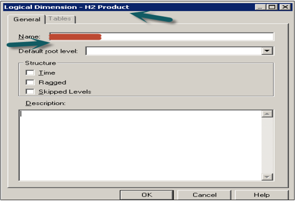
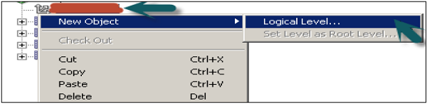
To create a logical level, right-click on logical dimension → New Object → Logical Level.
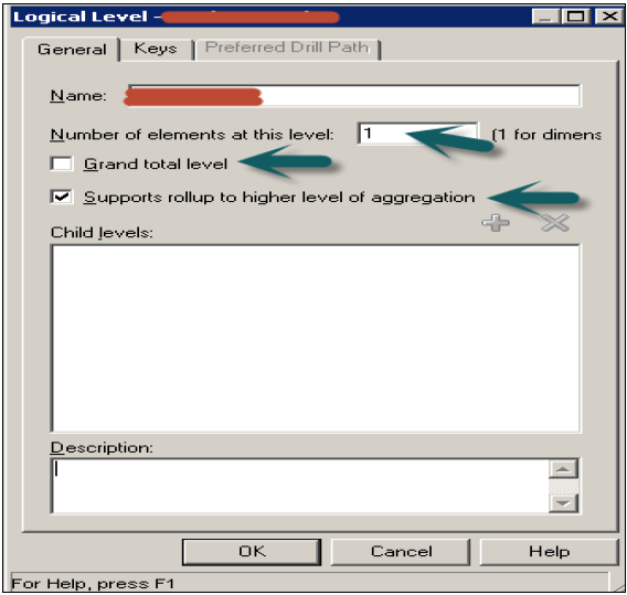
Enter the name of logical level example: Product_Name
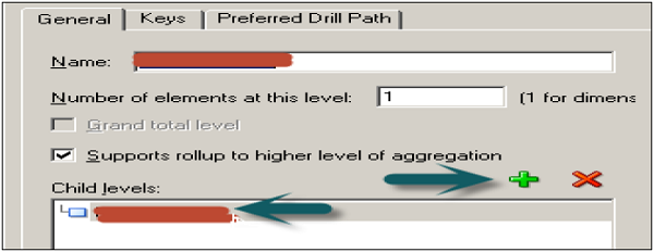
If this level is Grand total level, select the checkbox and the system will set number of element at this level to 1 by default → Click OK.
If you want the logical level to roll up to its parent, select the Supports rollup to parent elements checkbox → click OK.
If the logical level is not the grand total level and does not roll up, do not select any of the checkbox → Click OK.
Parent-Child Hierarchies
You can also add parent-child hierarchies in logical level by following these steps −
To define child logical levels, click Add in the Browse dialog box, select the child logical levels and click OK.
You can also right-click on logical level → New Object → Child level.
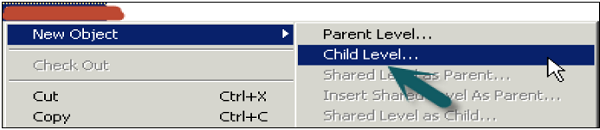
Enter the name of child level → Ok. You can repeat this to add multiple child levels for all logical columns as per requirement. You can also add Time and Region hierarchies in a similar way.
Now to add logical columns of a table to logical level → select logical column in BMM layer and drag it to logical level child name to which you want to map. Similarly you can drag all the columns of logical table to create parent-child hierarchies.
When you create a child level, it can be checked by a double-click on the logical level and it is displayed under child levels list of that level. You can add or delete child levels by using ‘+’ or ‘X’ option on top of this box.
Add Calculation to a Fact Table
Double-click on the column name in logical Fact table → Go to Aggregation tab and select the Aggregate function from the drop-down list → Click OK.
Measures represents data that is additive, such as total revenue or total quantity. Click on save option at the top to save the repository.
There are various Aggregate functions that can be used like Sum, Average, Count, Max, Min, etc.
OBIEE – Presentation Layer
Presentation layer is used to provide customized views of Business model in BMM layer to users. Subject areas are used in Presentation layer provided by Oracle BI Presentation Services.
There are various ways you can create subject areas in Presentation layer. Most common and simple method is by dragging Business Model in BMM layer to Presentation Layer and then making changes to it as per requirement.
You can move columns, remove or add columns in presentation layer so it allows you to make changes in a way that the user shouldn’t see columns that has no meaning for them.
Create Subject Areas/Presentation Catalogues and Presentation Tables in Presentation Layer
Right-click on Presentation area → New Subject Area → In General tab enter the name of subject area (Recommended similar to Business Model) → Click OK.
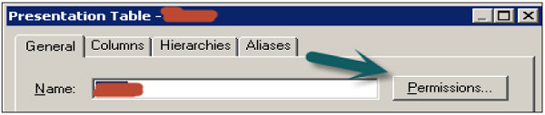
Once Subject area is created, right click on subject area → New Presentation table → in General tab, Enter name of presentation table → OK (Add number of presentation tables equal to number of parameters required in the report).

Click the Permissions tab → Permissions dialog box, where you can assign user or group permissions to the table.
Delete a Presentation Table
In the Presentation layer, right-click on subject Area → Presentation Catalog dialog box, click the Presentation Tables tab → Go to Presentation Tables tab, select a table and click Remove.
A confirmation message appears → Click Yes to remove the table or No to leave the table in the catalog → Click OK.
Move a Presentation Table
Go to Presentation Tables tab by a right-click on Subject Area → In the Name list, select the table you want to reorder → Use drag-and-drop to reposition the table or you can also use the Up and Down buttons to reorder the tables.
Presentation Columns Under Presentation Table
The name of presentation columns are normally same to the logical column names in the Business Model and Mapping layer. However, you can also enter a different name by unchecking Use Logical Column Name and the Display Custom Name in the Presentation Column dialog box.
Create Presentation Columns
The most simple way to create columns under Presentation tables is by dragging the columns from logical tables in BMM layer.
Select the objects under logical tables in BMM and drag them to Presentation tables under subject area (Use Ctrl key to select multiple objects for dragging). Repeat the process and add the logical columns to the remaining presentation tables.
Create a New Presentation Column −
Right-click on Presentation table in the Presentation layer → New Presentation Column.
Presentation Column dialog box appears. To use the name of the logical column, select the Use Logical Column checkbox.
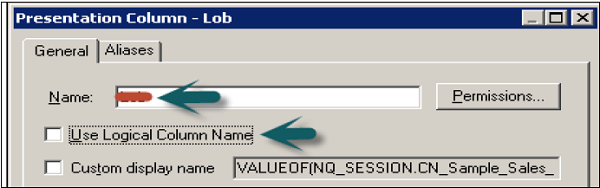
To specify a name that is different name, uncheck the Use Logical Column check box, and then type a name for the column.
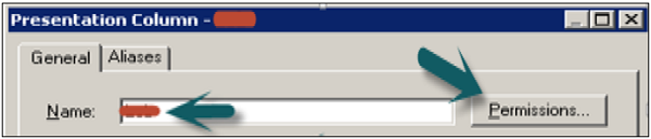
To assign user or group permissions to the column, click Permissions → In the Permissions dialog box, assign permissions → click OK.
Delete a Presentation Column
Right-click on presentation table in the Presentation layer → Click on Properties → Click on the Columns tab → Select the column you want to delete → Click Remove or press the Delete key →Click Yes.
To Reorder a Presentation Column
Right-click on presentation table in the Presentation layer → Go to Properties → Click the Columns tab → Select the column you want to reorder → Use drag-and-drop or you can also click Up and Down button → Click OK.

OBIEE – Testing Repository
You can check the repository for errors by using the consistency checking option. Once it is done, next step is to load the repository into Oracle BI Server. Then test the repository by running an Oracle BI analysis and verifying the results.
Go to File → click on Check Global Consistency → You will receive the following message → Click Yes.

Once you click OK → Business model under BMM will change to Green → Click on save the repository without checking global consistency again.
Disable Caching
To improve query performance, it is advised to disable BI server cache option.
Open a browser and enter the following URL to open Fusion Middleware Control Enterprise Manager: http://<machine name>:7001/em
Enter the user name and password. Click Login.
On the left side, expand Business Intelligence → coreapplication → Capacity Management tab → Performance.

Enable BI Server Cache section is by default checked → Click on Lock and Edit Configuration → Close.
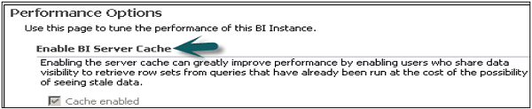
Now deselect cache enabled option. It is used to improve query performance. Go to Apply → Activate Changes → Completed Successfully.
Load the Repository
Go to Deployment tab → Repository → Lock and Edit Configuration → Completed Successfully.
Click on Upload BI Server Repository section → Browse to open the Choose file dialog box → select the Repository .rpd file and click Open → Enter Repository password → Apply → Activate Changes.
Activate Changes → Completed Successfully → Click on Restart to apply recent changes option at the top → Click Yes.
Repository is successfully created and loaded for query analysis.
Enable Query Logging
You can set up query logging level for individual users in OBIEE. Logging level controls the information that you will retrieve in log file.
Set Up Query Logging
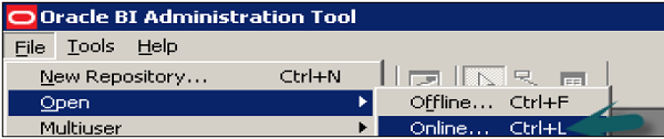
Open the Administration tool → Go to File → Open → Online.
Online mode is used to edit the repository in Oracle BI server. To open a repository in online mode, your Oracle BI server should be running.
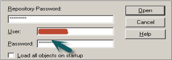
Enter the Repository password and user name password to login and click Open to open the repository.
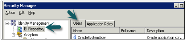
Go to Manage → Identity → Security Manager Window will open. Click BI Repository on the left side and double-click on Administrative user → User dialogue box will open.
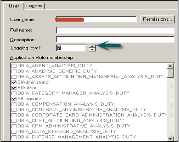
Click User tab in user dialogue box, you can set logging levels here.
In normal scenario − The user has a logging level set to 0 and the administrator has a logging level set to 2. Logging level can have values starting from Level 0 to level 5. Level 0 means no logging and Level 5 means maximum logging level information.
Logging Level Descriptions
| Level 0 | No logging |
| Level 1 | Logs the SQL statement issued from the client application Logs elapsed times for query compilation, query execution, query cache processing, and back-end database processing Logs the query status (success, failure, termination, or timeout). Logs the users ID, session ID, and request ID for each query |
| Level 2 | Logs everything logged in Level 1 Additionally, for each query, logs the repository name, business model name, presentation catalog (called Subject Area in Answer) name, SQL for the queries issued against physical databases, queries issued against the cache, number of rows returned from each query against a physical database and from queries issued against the cache, and the number of rows returned to the client application |
| Level 3 | Logs everything logged in Level 2
Additionally, adds a log entry for the logical query plan, when a query that was supposed to seed the cache was not inserted into the cache, when existing cache entries are purged to make room for the current query, and when the attempt to udate the exact match hit detector fails |
| Level 4 | Logs everything logged in Level 3 Additionally, logs the query execution plan. |
| Level 5 | Logs everything logged in Level 4 Additionally, logs intermediate row counts at various points in the execution plan. |
To Set Logging Level
In user dialogue box, enter value for logging level.
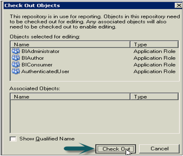
Once you click OK, it will open the checkout dialogue box. Click Checkout. Close the Security Manager.
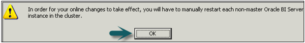
Go to file → Click on check-in changes → Save the repository using the Save option at the top → To take changes in effect → Click OK.
Use Query Log to Verify Queries
You can check query logs once query logging level is set by going to Oracle Enterprise Manager and this helps to verify queries.
To check the query logs to verify queries, go to Oracle Enterprise Manager OEM.
Go to diagnostic tab → click Log messages.
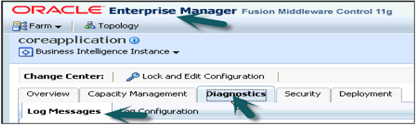
Scroll down to bottom in log messages to see Server, Scheduler, Action Services and other log details. Click on Server log to open log messages box.
You can select various filters − Date Range, Message types and message contains/not contains fields, etc. as shown in the following snapshot −
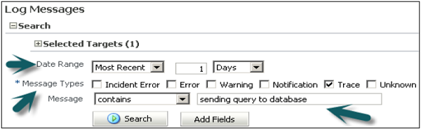
Once you click on search, it will show log messages as per filters.
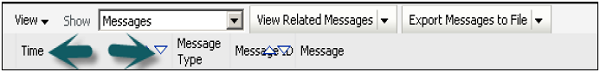
Clicking on collapse button allows you to check details of all log messages for queries.
OBIEE – Multiple Logical Table Sources
When you drag and drop a column from a physical table that is not currently being used in your logical table in BMM layer, the physical table containing such column gets added as a new Logical Table Source (LTS).
When in BMM layer, you use more than one table as source table, it is called multiple logical table sources. You can have a Fact table as multiple logical table sources when it uses different physical tables as source.
Example
Multiple LTS are used to convert Snowflakes schema to Star schemas in BMM layer.
Let us say you have two dimensions − Dim_Emp and Dim_Dept and one fact table FCT_Attendance in the Physical layer.
Here your Dim_Emp is normalized to Dim_Dept to implement Snowflakes schema. So in your Physical diagram, it would be like this −
Dim_Dept<------Dim_Emp <-------FCT_Attendance
When we move these table to the BMM layer, we will create a single dimension table Dim_Employee with 2 logical sources corresponding to Dim_Emp and Dim_Dept. In your BMM diagram −
Dim_Employee <-----------FCT_Attendance
This is one approach where you can use concept of multiple LTS in BMM layer.
Specifying Content
When you use multiple physical tables as sources, you expand table sources in BMM diagram. It shows all multiple LTS from where it is picking up the data in BMM layer.
To see table mapping in BMM layer, expand the sources under logical table in BMM layer. It will open Logical table source mapping dialogue box. You can check all tables which are mapped to provide data in logical table.
OBIEE – Calculation Measures
Calculated measures is used to perform calculation of facts in logical tables. It defines Aggregation functions in Aggregation tab of logical column in the repository.
Create New Measure
Measures are defined in logical fact tables in repository. Any column with an aggregation function applied on it is called a measure.
Common measure examples are − Unit Price, quantity sold, etc.
Following are the guidelines to create measures in OBIEE −
All aggregation should be performed from a fact logical table and not from a dimension logical table.
All columns that cannot be aggregated should be expressed in a dimension logical table and not in a fact logical table.
Calculated measures can be defined in two ways in logical tables at BMM layer in Administration tool −
- Aggregations in logical tables.
- Aggregations in logical table source.
Create Calculated Measures in Logical Tables using Administration Tool
Double-click on the column name in the logical Fact table, you will see the following dialog box.
Go to Aggregation tab and select the Aggregate function from the drop-down list → Click OK.

You can add new measures using functions in Expression builder wizard in Column source. Measures represent data that is additive, such as total revenue or total quantity. Click on the save option at the top to save the repository. This is also called creating measures at logical level.
Create Calculated Measures in Logical Table Source using Administration Tool
You can define Aggregations by a double-click on Logical table source to open logical table dialogue box.
Click on Expression builder wizard to define expression.
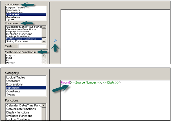
In Expression builder, you can choose multiple options like - Category, functions, and mathematical functions.
Once you select the category, it will show the subcategories inside it. Select the subcategory and mathematical function, and click on the arrow mark to insert it.
Now to edit the value to create measures, click on source number, enter the calculated value like multiple and divide → Go to Category and select logical table → Select column to apply this multiple/division to an existing column value.
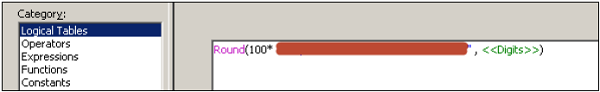
Click OK to close the Expression builder. Again click OK to close the dialog box.
OBIEE – Dimension Hierarchies
Hierarchies is a series of many-to-one relationships and can be of different levels. A Region hierarchy consists of: Region → Country → State → City → Street. Hierarchies follow top-down or bottom-up approach.
Logical dimensions or dimension hierarchies are created in BMM layer. There are two types of dimensional hierarchies that are possible −
- Dimensions with level-based hierarchies.
- Dimension with Parent-Child hierarchies.
In level-based hierarchies, members can be of different types and members of the same type come only at single level.
In Parent-Child hierarchies, all members are of the same type.
Dimensions with Level-based Hierarchies
Level-based dimension hierarchies can also contain parent-child relationships. The common sequence to create level-based hierarchies is to start with grand total level and then working down to lower levels.
Level-based hierarchies allows you to perform −
- Level-based calculated measures.
- Aggregate navigation.
- Drill down to child level in dashboards.
Each dimension can only have one grand total level and it doesn’t have a level key or dimension attributes. You can associate measures with grand total level and default aggregation for these measures are grand total always.
All lower levels should have at least one column and each dimension contains one or more hierarchies. Each lower level also contains a level key which defines unique value at that level.
Types of Level-based Hierarchies
Unbalanced Hierarchies
Unbalanced hierarchies are those where all the lower levels don’t have the same depth.
Example − For one product, for one month you can have data for weeks and for other month you can have data available for day level.
Skip Level Hierarchies
In skip-level hierarchies, few members don’t have values at higher level.
Example − For one city, you have state → country → Region. However for other city, you have only state and it doesn’t fall under any country or region.
Dimension with Parent-child Hierarchies
In parent-child hierarchy, all the members are of the same type. The most common example of parent-child hierarchy is the reporting structure in an organization. Parent-child hierarchy is based on a single logical table. Each row contains two keys – one for the member and another for the parent of the member.
OBIEE – Level-Based Measures
Level-based measures are created to perform calculation at a specific level of aggregation. They allow to return data at multiple levels of aggregation with one single query. It also allows to create share measures.
Example
Let us say there is a company XYZ Electronics which sells its products in many regions, countries and cities. Now the company President wants to see the total revenue at country level - one level below region and one level above cities. So total revenue measure should be summed up to the country level.
These type of measures are called level-based measures. Similarly, you can apply level-based measures on the time hierarchies.
Once the dimension hierarchies are created, level-based measures can be created by double clicking on the total revenue column in the logical table and setting the level in the levels tab.
Create Level-Based Measures
Open the repository in offline mode. Go to File → Open → Offline.
Select .rpd file and click open → Enter repository password and click Ok.
In BMM layer, right-click on Total Revenue column → New Object → Logical column.
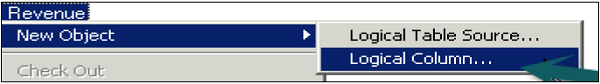
It will open the logical column dialog box. Enter the name of logical column total revenue. Go to column source tab → Check derived from existing columns using an expression.
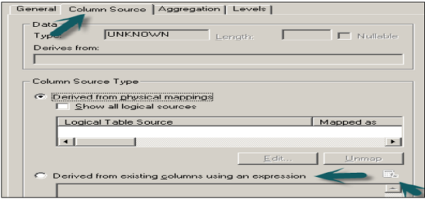
Once you select this option, expression edit wizard will be highlighted. In expression builder wizard, select the logical table → Column name → Total revenue from the left side menu → Click OK.
Now go to level tab in logical column dialog box → Click on logical dimension to select it as grand total under logical level. This specifies that the measure should be calculated at grand total level in the dimension hierarchy.
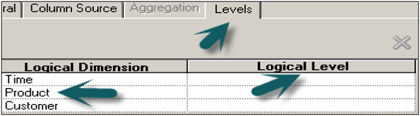
Once you click OK → Total Revenue logical table will appear under the logical dimension and Fact tables.
This column can be dragged to presentation layer in the subject area to be used by end users to generate reports. You can drag this column from fact tables or from logical dimension.
OBIEE – Aggregates
Aggregations are used to implement query performance optimization while running the reports. This eliminates the time taken by query to run the calculations and delivers the results at fast speed. Aggregate tables has less number of rows as compared to a normal table.
How Aggregation Works in OBIEE?
When you execute a query in OBIEE, BI server looks for the resources which has information to answer the query. Out of all available sources, the server selects the most aggregated source to answer that query.
Adding Aggregation in a Repository
Open the Repository in an offline mode in the Administrator tool. Go to File → Open → Offline.
Import the metadata and create logical table source in BMM layer. Expand the table name and click on source table name to open logical table source dialog box.
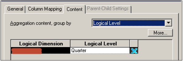
Go to column mapping tab to see map columns in Physical table. Go to content tab → Aggregate content group by selecting the logical level.
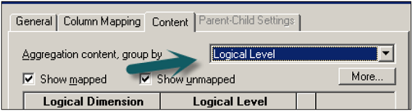
You can select different logical levels as per the columns in fact tables like Product Total, Total Revenue, and Quarter/Year for Time as per dimension hierarchies.
Click OK to close dialog box → save the repository.
When you define Aggregate in logical fact tables they are defined as per dimension hierarchies.
OBIEE – Variables
In OBIEE, there are two types of variables that are commonly used −
- Repository variables
- Session variables
Apart from this you can also define Presentation and Request variables.
Repository Variables
A Repository variable has a single value at any point of time. Repository variables are defined using Oracle BI Administration tool. Repository variables can be used in place of constants in Expression Builder Wizard.
There are two types of Repository variables −
- Static repository variables
- Dynamic repository variables
Static repository variables are defined in variable dialog box and their value exists until they are changed by the administrator.
Static repository variables contain default initializers that are numeric or character values. In addition, you can use Expression Builder to insert a constant as the default initializer, such as date, time, etc. You cannot use any other value or expression as the default initializer for a static repository variable.
In older BI versions, the Administrator tool did not limit value of static repository variables. You may get warning in consistency check if your repository has been upgraded from older versions. In such case, update the static repository variables so that default initializers have a constant value.
Dynamic repository variables are same as static variables but the values are refreshed by data returned from queries. When defining a dynamic repository variable, you create an initialization block or use a preexisting one that contains a SQL query. You can also set up a schedule that the Oracle BI Server will follow to execute the query and refresh the value of the variable periodically.
When the value of a dynamic repository variable changes, all cache entries associated with a business model are deleted automatically.
Each query can refresh several variables: one variable for each column in the query. You schedule these queries to be executed by the Oracle BI server.
Dynamic repository variables are useful for defining the content of logical table sources. For example, suppose you have two sources for information about orders. One source contains current orders and the other contains historical data.
Create Repository Variables
In the Administration Tool → Go to Manage → Select Variables → Variable Manager → Go to Action → New → Repository > Variable.
In the Variable dialog, type a name for the variable (Names for all variables should be unique) → Select the type of variable - Static or Dynamic.
If you select dynamic variable, use the initialization block list to select an existing initialization block that will be used to refresh the value on a continuing basis.
To create a new initialization block → Click New. To add a default initializer value, type the value in the default initializer box, or click the Expression Builder button to use Expression Builder.
For static repository variables, the value you specify in the default initializer window persists. It will not change unless you change it. If you initialize a variable using a character string, enclose the string in single quotes. Static repository variables must have default initializers that are constant values → Click OK to close the dialog box.
Session Variables
Session variables are similar to dynamic repository variables and they obtain their values from initialization blocks. When a user begins a session, the Oracle BI server creates new instances of session variables and initializes them.
There are as many instances of a session variable as there are active sessions on the Oracle BI server. Each instance of a session variable could be initialized to a different value.
There are two types of Session variables −
- System session variables
- Non-system session variables
System session variables are used by Oracle BI and Presentation server for specific purposes. They have predefined reserved names which can’t be used by other variables.
USER |
This variable holds the value the user enters with login name. This variable is typically populated from the LDAP profile of the user. |
USERGUID |
This variable contains the Global Unique Identifier (GUID) of the user and it is populated from the LDAP profile of the user. |
GROUP |
It contains the groups to which the user belongs. When a user belongs to multiple groups, include the group names in the same column, separated by semicolons (Example - GroupA;GroupB;GroupC). If a semicolon must be included as part of a group name, precede the semicolon with a backslash character (\). |
ROLES |
This variable contains the application roles to which the user belongs. When a user belongs to multiple roles, include the role names in the same column, separated by semicolons (Example - RoleA;RoleB;RoleC). If a semicolon must be included as part of a role name, precede the semicolon with a backslash character (\). |
ROLEGUIDS |
It contains the GUIDs for the application roles to which the user belongs. GUIDs for application roles are the same as the application role names. |
PERMISSIONS |
It contains the permissions held by the user. Example - oracle.bi.server.manageRepositories. |
Non-system session variables are used for setting the user filters. Example, you could define a non-system variable called Sale_Region that would be initialized to the name of the sale_region of the user.
Create Session Variables
In the Administration Tool → Go to Manage → Select Variables.
In the Variable Manager dialog, click Action → New → Session → Variable.
In the Session Variable dialog, enter variable name (Names for all variables should be unique and names of system session variables are reserved and cannot be used for other types of variables).
For session variables, you can select the following options −
Enable any user to set the value − This option is used to set session variables after the initialization block has populated the value. Example - this option lets non-administrators set this variable for sampling.
Security sensitive − This is used to identify the variable as sensitive to security when using a row-level database security strategy, such as a Virtual Private Database (VPD).
You can use the initialization block list option to choose an initialization block that will be used to refresh the value regularly. You can also create a new initialization block.
To add a default initializer value, enter the value in the default initializer box or click the Expression Builder button to use Expression Builder. Click OK to close the dialog box.
The administrator can create non-system session variables using Oracle BI Administration tool.
Presentation Variables
Presentation variables are created with creation of Dashboard prompts. There are two types of dashboard prompts that can be used −
Column Prompt
Presentation variable created with column prompt is associated with a column, and the values that it can take comes from the column values.
To create a presentation variable go to New Prompt dialog or Edit Prompt dialog → Select Presentation Variable in the Set of a variable field → Enter the name for the variable.
Variable Prompt
Presentation variable created as variable prompt is not associated with any column and you need to define its values.
To create a presentation variable as part of a variable prompt, in the New Prompt dialog or Edit Prompt dialog → Select Presentation Variable in the Prompt for field → Enter the name for the variable.
The value of a presentation variable is populated by the column or variable prompt with which it is created. Each time a user selects a value in the column or variable prompt, the value of the presentation variable is set to the value that the user selects.
Initialization Blocks
Initialization blocks are used to initialize OBIEE variables: Dynamic Repository variables, system session variables and non-system session variables.
It contains SQL statement that are executed to initialize or refresh the variables associated with that block. The SQL statement that are executed points to physical tables that can be accessed using the connection pool. Connection pool is defined in the initialization block dialog.
If you want the query for an initialization block to have database-specific SQL, you can select a database type for that query.
Initialize Dynamic Repository Variables using Initialization Block
Default initiation string field of initialization block is used to set value of dynamic repository variables. You also define a schedule which is followed by Oracle BI server to execute the query and refresh the value of variable. If you set the logging level to 2 or higher, log information for all SQL queries executed to retrieve the value of variable is saved in nqquery.log file.
Location of this file on BI Server −
ORACLE_INSTANCE\diagnostics\logs\OracleBIServerComponent\coreapplication_obisn
Initialize Session Variables using Initialization Block
Session variables also take their values from initialization block but their value never changes with time intervals. When a user begins a new session, Oracle BI server creates a new instance of session variables.
All SQL queries executed to retrieve session variable information by BI server if the logging level is set to 2 or higher in the Identity Manager User object or the LOGLEVEL system session variable is set to 2 or higher in the Variable Manager is saved in nqquery.log file.
Location of this file on BI Server −
ORACLE_INSTANCE\diagnostics\logs\OracleBIServerComponent\coreapplication_obisn
Create Initialization Blocks in Administrator Tool
Go to Manager → Variables → Variable Manager Dialog box appears. Go to Action menu → Click New → Repository → Initialization Block → Enter the name of initialization block.
Go to Schedule tab → Select start date and time and refresh interval.
You can choose the following options for Initialization Blocks −
Disable − If you select this option, initialization block is disabled. To enable an initialization block, right-click an existing initialization block in the Variable Manager and choose Enable. This option enables you to change this property without opening the initialization block dialog.
Allow deferred execution − This allows you to defer the execution of the initialization block until an associated session variable is accessed for the first time during the session.
Required for authentication − If you select this, initialization block must execute for users to log in. Users are denied access to Oracle BI if the initialization block doesn’t execute.
OBIEE – Dashboards
OBIEE dashboard is a tool that enables end users to run ad-hoc reports and analysis as per business requirement model. Interactive dashboards are pixel perfect reports which can be directly viewed or printed by end users.
OBIEE dashboard is part of Oracle BI Presentation layer services. If your end user is not interested in seeing all the data in the dashboard, it allows you to add prompts to the dashboard that allows the end user to enter what he wants to see. Dashboards also allow end users to select from drop-down lists, multi-select boxes and selection of columns to display in the reports.
Dashboard Alerts
Oracle BI dashboard allows you to set up alerts for sales executives that comes up on the interactive dashboard whenever the company’s projected sales is going to be below forecast.
Create a New Dashboard
To create a new Dashboard, go to New → Dashboard or you can also click on Dashboard option under create on the left side.
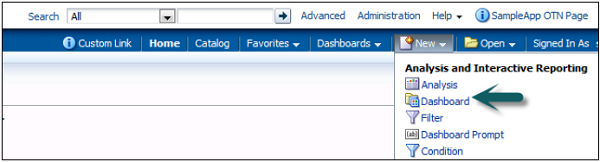
Once you click on Dashboard, new dashboard dialog box opens up. Enter the name of Dashboard and description and select the location where you want Dashboard to save → click OK.
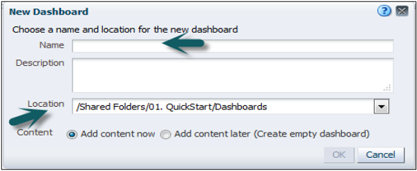
If you save the dashboard in the Dashboards subfolder directly under the /Shared Folders/first level subfolder → dashboard will be listed in the Dashboard menu on the global header.
If you save it in a Dashboards subfolder at any other level (such as /Shared Folders/Sales/Eastern), it will not be listed.
If you choose a folder in the Dashboards subfolder directly under the /Shared Folders/first level subfolder in which no dashboards have been saved, a new Dashboards folder is automatically created for you.
Once you enter the above fields, Dashboard builder will open up as shown in the following snapshot −
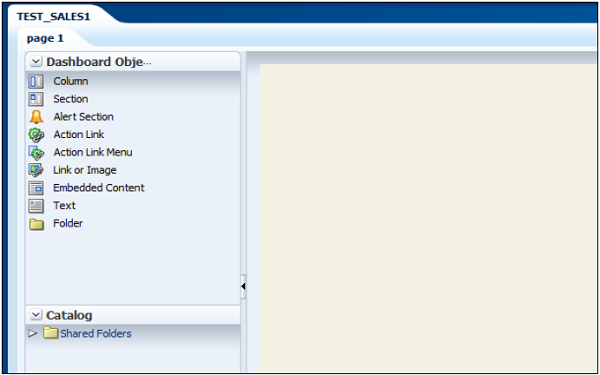
Expand the catalog tab, select analysis to add to Dashboard and drag to page layout pane. Save and run the dashboard.
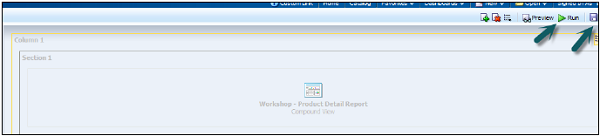
Edit a Dashboard
Go to Dashboard → My Dashboard → Edit Dashboard.
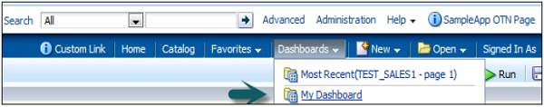
To edit Dashboard. Click on below icon → Dashboard properties.
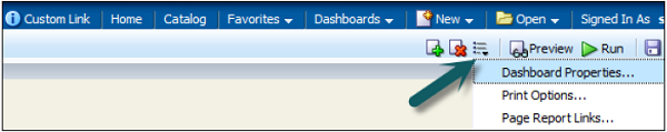
A new dialog box will appear as shown in the following snapshot. You can perform the following tasks −
Change the styles (Styles control how dashboards and results are formatted for display, such as the color of text and links, the font and size of text, the borders in tables, the colors and attributes of graphs, and so on). You can add a description.
You can add hidden prompts, filters, and variables. Specify the links that will display with analyses on a dashboard page. You can rename, hide, reorder, set permissions for, and delete dashboard pages.
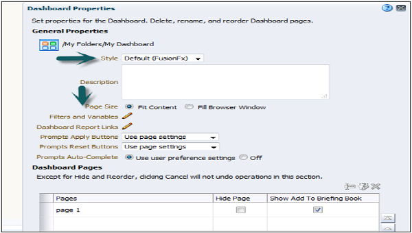
You can also edit Dashboard page properties by selecting page in the dialog box. You can make the following changes −
You can change the name of your dashboard page.
You can add a hidden prompt. Hidden prompts are used to set default values for all corresponding prompts on a dashboard page.
You can add permissions for the dashboard and can also delete the selected page. Dashboard pages are permanently deleted.
If more than one dashboard page is in this dashboard, the arrange order icons are enabled using up and down arrows.
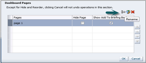
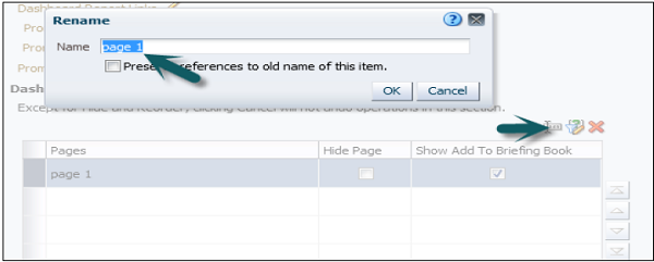
To set the report links at the dashboard level, dashboard page, or analysis level click the edit option of Dashboard reporting links.
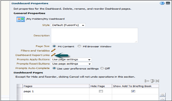
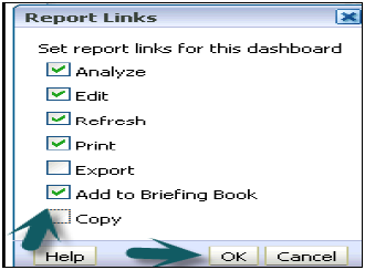
To add a dashboard page, click on new Dashboard page icon → Enter the name of dashboard page and click OK.
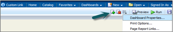
In Catalog tab, you can add the new another analysis and drag it to page layout area of new dashboard page.
To edit the properties of dashboard like cell width, border, and height, click on column properties. You can set background color, wrap text and additional formatting options.
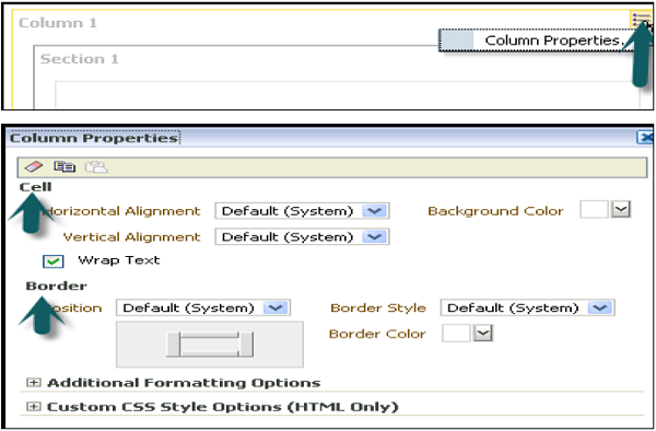
You can also add a condition on dashboard data display by clicking on condition option in column properties −
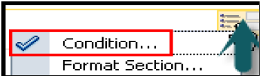
To add a condition, click on + sign in condition dialog box. You can add a condition based on analysis.
Select the condition data and enter the condition parameter.
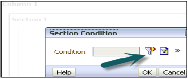
You can also test, edit or remove the condition by clicking on ‘more’ sign next to + button.
Save a Customized Dashboard
You can save your customized dashboard by going to page options → Save current customizations → Enter the name of customization → Click OK.
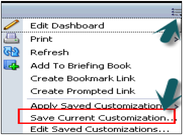
To apply customization to a dashboard page, go to page option → Apply saved customization → Select name → Click OK.
It allows you to save and view dashboard pages in their current state such as filters, prompts, column sorts, drills in analyses, and section expansion and collapse. By saving customizations, you do not need to make these choices manually each time you access the dashboard page.
OBIEE – Filters
Filters are used to limit the results that are displayed when an analysis is run, so that the results answer a particular question. Based on the filters, only those results are shown that matches the criteria passed in the filter condition.
Filters are applied directly to attribute and measure columns. Filters are applied before the query is aggregated and affect the query and thus the resulting values for measures.
For example, you have a list of members in which the aggregate sums to 100. Over time, more members meet the set filter criteria, which increases the aggregate sum to 200.
Column Filters
Following are the ways to create filters −
Create a Named Column Filter
Go to Oracle Business Intelligence homepage → New menu → Select filter. The Select Subject Area dialog is displayed.
From the Select Subject Area dialog, choose the subject area for which you want to create a filter. The "Filter editor" is displayed from the "Subject Areas pane". Double-click the column for which you want to create the filter. New Filter dialog is displayed.
Create an Inline Filter
Either create an analysis or access an existing analysis for which you want to create a filter.
Click the Criteria tab → Locate the "Filters pane" → Click create a filter for the current subject area button. The analysis selected columns are displayed in the cascading menu.
Select a column name from the menu or select the More Columns option to access the “Select Column dialog" from which you can select any column from the subject area.
Once you select a column, the "New Filter dialog" is displayed.
OBIEE – Views
Oracle BI Enterprise Edition enables you to look at results of analyses in a meaningful way using its presentation capabilities. Different types of views can be added, such as graphs and pivot tables that allow drilling down to more detailed information and many more options like using filters, etc.
The results of the analysis is displayed using a table/Pivot table view and depends on the type of columns that the analysis contains −
Table view is used if the analysis contains only attribute columns/only measure columns or a combination of both.
Pivot table is the default view if the analysis contains at least one hierarchical column.
A title view displays the name of the saved analysis.
You can edit or delete an existing view, add another view to an analysis and can also combine views.
Types of Views
| Sr.No | Views & Description |
|---|---|
| 1 |
Title Title view displays a title, a subtitle, a logo, a link to a custom online help page and timestamps to the results. |
| 2 |
Table Table view is used to display results in a visual representation of data organized by rows and columns. It provides a summary view of data and enables users to see different views of data by dragging and dropping rows and columns. |
| 3 |
Pivot Table It displays results in a pivot table, which provides a summary view of data in cross-tab format and enables users to see different views of data by dragging and dropping rows and columns. Pivot tables and standard tables are similar in structure but Pivot table can contain column groups and can also display multiple levels of both row and column headings. Pivot table cell contains a unique value. Pivot table is more efficient than a row-based table. It is best suited for displaying a large quantity of data, for browsing data hierarchically, and for trend analysis. |
| 4 |
Performance Tile Performance tiles are used to display a single aggregate measure value in a manner that is visually simple but provides a summary metrics to the user that will likely be presented in more detail within a dashboard view. Performance tiles are used to focus the user's attention on simple, need-to-know facts directly and prominently on the tile. Communicate status through simple formatting by using color, labels, and limited styles, or through conditional formatting of the background color or measure value to make the tile visually prominent. For example, if revenue is not tracking to target, the revenue value may appear in red. Respond to prompts, filters, and user roles and permissions by making them relevant to the user and their context. Support a single, aggregate or calculated value. |
| 5 |
Treemap Tree map are used to display a space-constrained, 2-d visualization for hierarchical structures with multiple levels. Treemaps are limited by a predefined area and display two levels of data. Contain rectangular tiles. The size of the tile is based on a measure, and the color of the tile is based on a second measure. Treemap are similar to a scatter plot graphs in that the map area is constrained, and the graph allows you to visualize large quantities of data and quickly identify trends and anomalies within that data. |
| 6 |
Trellis Trellis displays multi-dimensional data shown as a set of cells in a grid form and where each cell represents a subset of data using a particular graph type. The trellis view has two subtypes − Simple Trellis and Advanced Trellis. Simple trellis views are ideal for displaying multiple graphs that enable comparison of like to like. Advanced trellis views are ideal for displaying spark graphs that show a trend. A simple trellis displays a single inner graph type, Example − a grid of multiple Bar graphs. An advanced trellis displays a different inner graph type for each measure. Example: A mixture of Spark Line graphs and Spark Bar graphs, alongside numbers. |
| 7 |
Graph Graph displays numeric information visually which makes it easier to understand large quantities of data. Graphs often reveal patterns and trends that text-based displays cannot. A graph is displayed on a background, called the graph canvas. |
| 8 |
Gauge Gauge are used to show a single data value. Cos of its compact size, a gauge is often more effective than a graph for displaying a single data value Gauges identify problems in data. A gauge usually plots one data point with an indication of whether that point falls in an acceptable or unacceptable range. Thus, gauges are useful for showing performance against goals. A gauge or gauge set is displayed on a background, called the gauge canvas. |
| 9 |
Funnel Funnel displays results in 3D graph that represents target and actual values using volume, level, and color. Funnel graphs are used to graphically represent data that changes over different periods or stages. Example: Funnel graphs are often used to represent the volume of sales over a quarter. Funnel graphs are well suited for showing actual compared to targets for data where the target is known to decrease (or increase) significantly per stage, such as a sales pipeline. |
| 10 |
Map view Map view is used to display results overlain on a map. Depending on the data, the results can be overlain on top of a map as formats such as images, color fill areas, bar and pie graphs, and variably sized markers. |
| 11 |
Filters Filter are used to displays the filters in effect for an analysis. Filters allows you to add condition to an analysis to obtain results that answer a particular question. Filters are applied before the query is aggregated. |
| 12 |
Selection Steps Selection steps are used to displays the selection steps in effect for an analysis. Selection steps, like filters, allow you to obtain results that answer particular questions. Selection steps are applied after the query is aggregated. |
| 13 |
Column Selector Column selector is a set of drop-down lists that contain pre-selected columns. Users can dynamically select columns and change the data that is displayed in the views of the analysis. |
| 14 |
View Selector A view selector is a drop-down list from which users can select a specific view of the results from among the saved views. |
| 15 |
Legend It enables you to document the meaning of special formatting used in results-meaning of custom colors applied to gauges. |
| 16 |
Narrative It displays the results as one or more paragraphs of text. |
| 17 |
Ticker It displays the results as a ticker or marquee, similar in style to the stock tickers that run across many financial and news sites on the Internet. You can also control what information is presented and how it scrolls across the page. |
| 18 |
Static Text You can use HTML to add banners, tickers, ActiveX objects, Java applets, links, instructions, descriptions, graphics, etc. in the results. |
| 19 |
Logical SQL It displays the SQL statement that is generated for an analysis. This view is useful for trainers and administrators, and is usually not included in results for typical users. You cannot modify this view, except to format its container or to delete it. |
| 20 |
Create Segment It is used to display a Create Segment link in the results. |
| 21 |
Create Target List It is used to display a create target list link in the results. Users can click this link to create a target list, based on the results data, in their Oracle's Siebel operational application. This view is for users of Oracle's Siebel Life Sciences operational application integrated with Oracle's Siebel Life Sciences Analytics applications. |
All view types except logical SQL view can be edited. Each view has its own editor in which you can perform edit task.
Each view editor contains a unique functionality for that view type but might also contain functionality that is the same across view types.
Edit a View
Open the analysis that contains the view to edit. Click the "Analysis editor: Results tab."
Click the Edit View button for the view. View editors is displayed. Now, using the editor for the view, make the required edits. Click done and then save the view.
Delete a View
You can delete a view from −
A compound layout − If you remove a view from a compound layout, it is only removed from the compound layout and not from the analysis.
An analysis − If you remove a view from an analysis, it removes the view from the analysis and also from any compound layout to which it had been added.
Remove a View
If you want to remove a view from −
A compound layout − In the view in the Compound Layout → click the Remove View from Compound Layout button.
An analysis − In the Views pane → select the view and then click the Remove View from Analysis toolbar button.
OBIEE – Prompts
A Prompt is a special type of filter that is used to filter analyses embedded in a dashboard. The main reason to use a dashboard prompt is that it allows the user to customize analysis output and also allows flexibility to change parameters of a report. There are three types of prompts that can be used −
Named Prompts
The prompt created at the dashboard level is called a Named prompt. This Prompt is created outside of a specific dashboard and stored in the catalog as a prompt. You can apply a named prompt to any dashboard or dashboard page that contains the columns, mentioned in the prompt. It can filter one or any number of analyses embedded on the same dashboard page. You can create and save these named prompts to a private folder or a shared folder.
A named prompt always appears on the dashboard page and the user can prompt for different values without having to rerun the dashboard. A named prompt can also interact with selection steps. You can specify a dashboard prompt to override a specific selection step.
The step will be processed against the dashboard column with the user-specified data values collected by the dashboard column prompt, whereas all other steps will be processed as originally specified.
Inline Prompts
Inline prompts are embedded in an analysis and are not stored in the catalog for reuse. Inline prompt provides general filtering of a column within the analysis, depending on how it is configured.
Inline prompt works independently from a dashboard filter, which determines values for all matching columns on the dashboard. An inline prompt is an initial prompt. When the user selects the prompt value, the prompt field disappears from the analysis.
To select different prompt values, you need to rerun the analysis. Your input determines the content of the analyses embedded in the dashboard.
Named Prompt can be applied to any dashboard or dashboard page which contains the column specified in the Prompt.
Column Prompts
A column prompt is the most common and flexible prompt type. A column prompt enables you to build very specific value prompts to either stand alone on the dashboard or analysis or to expand or refine existing dashboard and analysis filters. Column prompts can be created for hierarchical, measure, or attribute columns at the analysis or dashboard level.
Go to New → Dashboard Prompt → Select subject area.
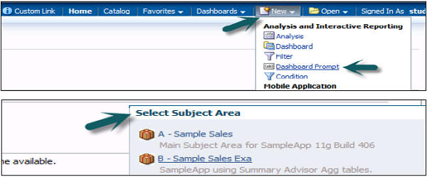
Dashboard prompt dialog box appears. Go to ‘+’ sign, select the prompt type. Click on the column prompt → Select column → Click OK.
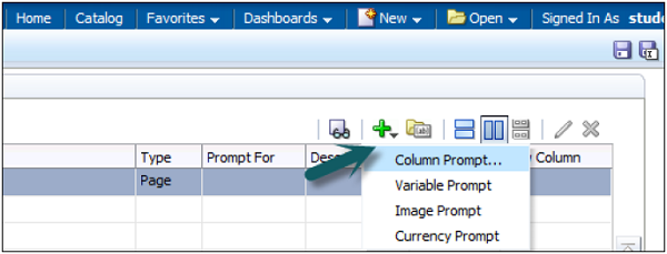
New Prompt dialog box appears (this appears only for column prompts). Enter the label name that will appear on dashboard next to Prompt → Select the Operator → User Input.
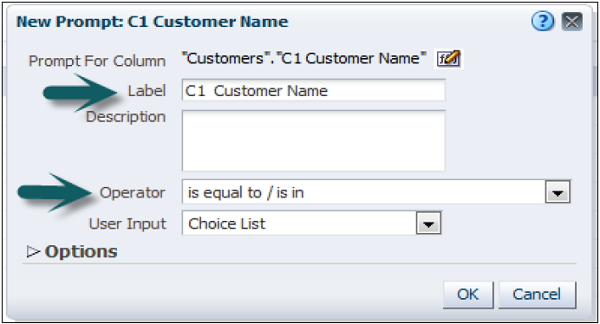
The User Input field's drop-down list appears for column and variable prompts, and provides you with the option to determine the User Input method for the user interface. You can select any of the following − checkboxes, radio buttons, a choice list, or a list box.
Example − If you select the User Input method of Choice List and Choice List Values item of all Column Values, the user will select the prompt's data value from a list that contains all of the data values contained in the data source.
You can also further make a selection by expanding the Options tab.
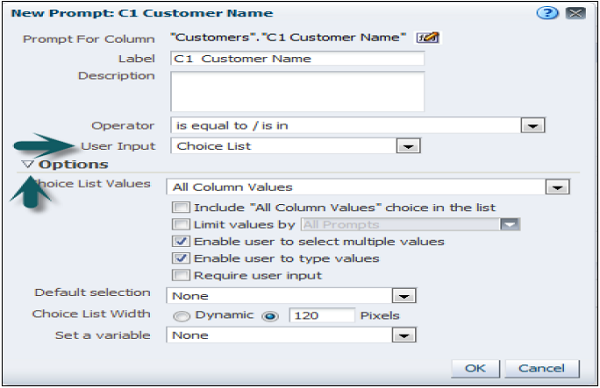
These series of checkboxes allow you to restrict the amount of data returned in output. Once selection is made, click OK.
The Prompt is added to Definition → Save the prompt using the save option at the top right corner → Enter the name → Click OK.
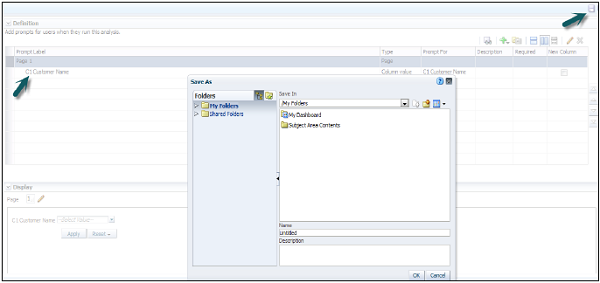
To test the Prompt, go to My Dashboard → Catalog and drag the prompt to column 1. This prompt can be applied to full dashboard or on a single page by clicking on Properties → Scope.
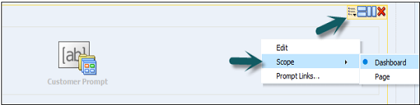
Save and run the Dashboard, select the value for a Prompt. Apply and Output value will change as per prompt value.
Other Prompts
Currency Prompt
A currency prompt enables the user to change the currency type that is displayed in the currency columns on an analysis or dashboard.
Example − Suppose that an analysis contains the sales totals for a certain region of US in US dollars. However, because the users viewing the analysis reside in Canada, they can use the currency prompt to change the sales totals from USD to Canada dollars.
The prompt's currency selection list is populated with the currency preferences from the user’s → My Account dialog → Preferences tab. Currency prompt option is available only if the administrator has configured the userpref_currencies.xml file.
Image Prompt
An image prompt provides an image that users click to select values for an analysis or dashboard.
Example − In a sales organization, users can click their territories from an image of a map to see sales information, or click a product image to see sales information about that product. If you know how to use the HTML <map> tag, then you can create an image map definition.
Variable Prompt
A variable prompt enables the user to select a value that is specified in the variable prompt to display on dashboard. A variable prompt is not dependent upon a column, but can still use a column.
Add Reports to BI Dashboard Pages
You can add one or more existing reports to a dashboard page. The advantage is that you can share reports with other users and schedule the dashboard pages using agents. An agent sends the entire dashboard to the user, including all data pages that the report references.
When configuring an agent for a dashboard page that contains a BI Publisher report, ensure that the following criteria are met −
- The output format of the BI Publisher report must be PDF.
- The agent must be set to deliver PDF.
You can add reports to a dashboard page as embedded content and as a link. Embedded means that the report is displayed directly on the dashboard page. The link opens the report in BI Publisher within Oracle BIEE.
If you modify the report in BI Publisher and save your changes, then refresh the dashboard page to see the modifications. Navigate to the page to which you want to add a report.
Add a BI Report to a Dashboard Page
Select a report in one of the following ways −
Select the report from the Catalog pane and drag and drop it into a section on the dashboard page.
To add a report from a dashboard page, select the report from the folder that contains its dashboard in the Catalog pane.
Set the properties of the object. To do so, hover the mouse pointer over the object in the page layout area to display the object's toolbar, and click the Properties button.
The "BI Publisher Report Properties dialog" is displayed. Complete the fields in the properties dialog as appropriate. Click OK and then click Save.
If required, add a prompt to the dashboard page to filter the results of an embedded parameterized report.
OBIEE – Security
OBIEE security is defined by the use of a role-based access control model. It is defined in terms of roles that are aligned to different directory server groups and users. In this chapter, we will be discussing the components defined to compose a security policy.
One can define a Security structure with the following components
The directory Server User and Group managed by the Authentication provider.
The application roles managed by the Policy store provide Security policy with the following components: Presentation catalog, repository, policy store.
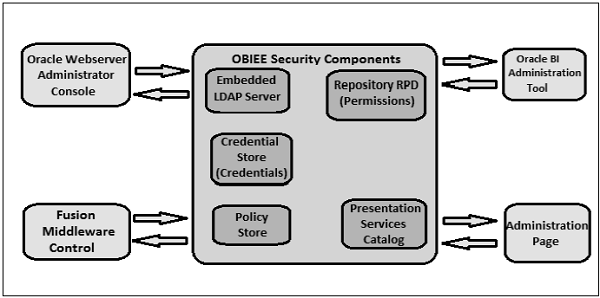
Security Providers
Security provider is called in order to get the security information. Following types of security providers are used by OBIEE −
Authentication provider to authenticate users.
Policy store provider is used to give privileges on all applications except for BI Presentation Services.
Credential store provider is used to store credentials used internally by the BI application.
Security Policy
Security policy in OBIEE is divided into the following components −
- Presentation Catalog
- Repository
- Policy Store
Presentation Catalog
It defines the catalog objects and Oracle BI Presentation Services functionality.
Oracle BI Presentation Services Administration
It enables you to set privileges for users to access features and functions such as editing views and creating agents and prompts.
Presentation Catalog privileges access to presentation catalog objects defined in the Permission dialog.
Presentation Services administration does not have its own authentication system and it relies on the authentication system that it inherits from the Oracle BI Server. All users who sign in to Presentation Services are granted the Authenticated User role and any other roles that they were assigned in Fusion Middleware Control.
You can assign permissions in one of the following ways −
To application roles − Most recommended way of assigning permissions and privileges.
To individual users − This is difficult to manage where you can assign permissions and privileges to specific users.
To Catalog groups − It was used in previous releases for backward compatibility maintenance.
Repository
This defines which application roles and users have access to which items of metadata within the repository. The Oracle BI Administration Tool through the security manager is used and enables you to perform the following tasks −
- Set permissions for business models, tables, columns, and subject areas.
- Specify database access for each user.
- Specify filters to limit the data accessible by users.
- Set authentication options.
Policy Store
It defines BI Server, BI Publisher, and Real Time Decisions functionality that can be accessed by given users or users with given Application Roles.
Authentication and Authorization
Authentication
Authenticator Provider in Oracle WebLogic Server domain is used for user authentication. This authentication provider accesses users and group information stored in the LDAP server in the Oracle Business Intelligence's Oracle WebLogic Server domain.
To create and manage users and groups in an LDAP server, Oracle WebLogic Server Administration Console is used. You can also choose to configure an authentication provider for an alternative directory. In this case, Oracle WebLogic Server Administration Console enables you to view the users and groups in your directory; however, you need to continue to use the appropriate tools to make any modifications to the directory.
Example − If you reconfigure Oracle Business Intelligence to use OID, you can view users and groups in Oracle WebLogic Server Administration Console but you must manage them in OID Console.
Authorization
Once authentication is done, the next step in security is to ensure that the user can do and see what they are authorized to do. Authorization for Oracle Business Intelligence 11g is managed by a security policy in terms of Applications Roles.
Application Roles
Security is normally defined in terms of Application roles that are assigned to directory server users and groups. Example: the default Application roles are BIAdministrator, BIConsumer, and BIAuthor.
Application roles are defined as functional role assigned to a user, which gives that user the privileges required to perform that role. Example: Marketing Analyst Application role might grant a user access to view, edit and create reports on a company's marketing pipeline.
This communication between Application roles and directory server users and groups allows the administrator to define the Application roles and policies without creating additional users or groups in LDAP server. Application roles allows business intelligence system to be easily moved between development, test and production environments.
This doesn’t require any change in security policy and all that is required is to assign the Application roles to the users and groups available in the target environment.
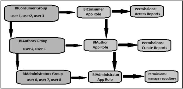
The group named 'BIConsumers' contains user1, user2, and user3. Users in the group 'BIConsumers' are assigned the Application role 'BIConsumer', which enables the users to view reports.
The group named 'BIAuthors' contains user4 and user5. Users in the group 'BIAuthors' are assigned the Application role 'BIAuthor', which enables the users to create reports.
The group named 'BIAdministrators' contains user6 and user7, user 8. Users in the group 'BIAdministrators' are assigned the Application role 'BIAdministrator', which enables the users to manage repositories.
OBIEE – Administration
In OBIEE 10g, most of OBIEE administration tasks were mostly performed either through the Administration tool, the web-based Presentation Server administration screen, or through editing files in the filesystem. There were around 700 or so configuration options spread over multiple tools and configuration files, with some options like users and groups were embedded in unrelated repositories (the RPD).
In OBIEE 11g, all administration and configuration tasks are moved into Fusion Middleware Control also called as Enterprise Manager.
Administration tool that was present in OBIEE 10g is also present in 11g and is used to maintain the semantic model used by the BI Server. It has few enhancements in terms of dimension handling and new data sources. A major change is around security - when you open the Security Manager dialog −
Go to Manage → Identity → Security Manager Dialog box appears.
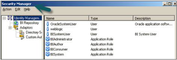
Users and Application Roles are now defined in the WebLogic Server admin console. You use the Security Manager to define additional links through to other LDAP servers, register custom authenticators and set up filters, etc. In the above screenshot, the users shown in the users list are those that are held in WebLogic Server’s JPS (Java Platform Security) service, and there are no longer any users and groups in the RPD itself.
There is no administrator user in above snapshot. It has standard administrator user that you set up as the WebLogic Server administrator when you install OBIEE, which typically has the username weblogic.
There are also two additional default users: OracleSystemUser - this user is used by the various OBIEE web services to communicate with the BI Server and BISystemUser is used by BI Publisher to connect to the BI Server as a data source.
In Application Roles tab, you can see a list default application roles - BISystem, BIAdministrator, BIAuthor and BIConsumer - which are used to grant access to Presentation Server functionality.
Create a User in OBIEE
To create a new user, log on to the WebLogic Server admin console → Go to Security Realms from the Fusion Middleware Control menu → Select myrealm → Select Users and Groups. Click on Users tab, it will show you a list of existing users.
Click the New. → New user dialog box opens up → enter the user’s details. You can also use the Groups tab to define a group for the user, or assign the user to an existing group.
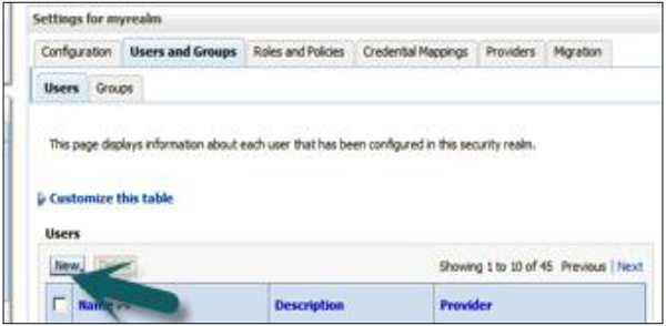
Configuration and Metadata Files
Following are the key file locations In OBIEE 11g −
RPD Directory
C:\Middleware\instances\instance1\bifoundation\OracleBIServerComponent\
coreapplication_obis1\repository
NQSConfig.INI
C:\Middleware\instances\instance1\config\OracleBIServerComponent\coreapplication_obis1\
nqsconfig.INI
NQClusterConfig.INI
C:\Middleware\instances\instance1\config\OracleBIApplication\coreapplication\
NQClusterConfig.INI
nqquery.log
C:\Middleware\instances\instance1\diagnostics\logs\OracleBIServerComponent\
coreapplication_obis1\nqquery.log
nqserver.log
C:\Middleware\instances\instance1\diagnostics\logs\OracleBIServerComponent\
coreapplication_obis1\nqserver.log
nqsserver.exe
C:\Middleware\Oracle_BI1\bifoundation\server\bin\nqsserver.exe
WebCat Directory
C:\Middleware\instances\instance1\bifoundation\OracleBIPresentationServicesComponent\
coreapplication_obips1\catalog\
instanceconfig.xml
C:\Middleware\instances\instance1\config\OracleBIPresentationServicesComponent\
coreapplication_obips1\instanceconfig.xml
xdo.cfg
C:\Middleware\instances\instance1\config\OracleBIPresentationServicesComponent\
coreapplication_obips1\xdo.cfg
sawlog0.log
C:\Middleware\instances\instance1\diagnostics\logs\OracleBIPresentationServicesComponent\
coreapplication_obips1\sawlog0.log
sawserver.exe
C:\Middleware\Oracle_BI1\bifoundation\web\bin\sawserver.exe
Go to Overview. You can also stop, start and restart all of the system components like BI Server, Presentation Server etc. via OPMN.
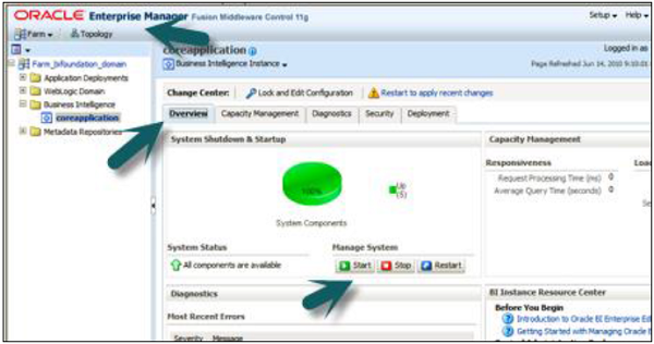
You can click the Capacity Management, Diagnostics, Security or Deployment tabs to perform further maintenance.
Capacity Management
We have the following four options available for capacity management −
Metrics gathered via DMS.
Availability of all the individual system components (allowing you to stop, start and restart them individually).
Scalability is used to increase the number of BI Servers, Presentation Servers, Cluster Controllers and Schedulers in the cluster in conjunction with the “scale out” install option.
Performance option allows you to turn caching on or off and modify other parameters associated with response time.
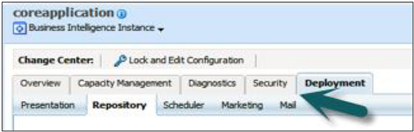
Diagnostics − Log Messages show you view of all server errors and warnings. Log Configuration allows you to limit the size of logs and information gets included in them.
Security − It is used for enabling SSO and selecting the SSO provider.
Deployment − Presentation allows you to set dashboard defaults, section headings, etc. Scheduler is used to set the connection details for the scheduler schema. Marketing is for configuring the Siebel Marketing Content Server connection. Mail option is used for setting up the mail server to deliver for email alerts. Repository is used to upload new RPDs for use by the BI Server.