- Machine Learning Basics
- Machine Learning - Home
- Machine Learning - Getting Started
- Machine Learning - Basic Concepts
- Machine Learning - Python Libraries
- Machine Learning - Applications
- Machine Learning - Life Cycle
- Machine Learning - Required Skills
- Machine Learning - Implementation
- Machine Learning - Challenges & Common Issues
- Machine Learning - Limitations
- Machine Learning - Reallife Examples
- Machine Learning - Data Structure
- Machine Learning - Mathematics
- Machine Learning - Artificial Intelligence
- Machine Learning - Neural Networks
- Machine Learning - Deep Learning
- Machine Learning - Getting Datasets
- Machine Learning - Categorical Data
- Machine Learning - Data Loading
- Machine Learning - Data Understanding
- Machine Learning - Data Preparation
- Machine Learning - Models
- Machine Learning - Supervised
- Machine Learning - Unsupervised
- Machine Learning - Semi-supervised
- Machine Learning - Reinforcement
- Machine Learning - Supervised vs. Unsupervised
- Machine Learning Data Visualization
- Machine Learning - Data Visualization
- Machine Learning - Histograms
- Machine Learning - Density Plots
- Machine Learning - Box and Whisker Plots
- Machine Learning - Correlation Matrix Plots
- Machine Learning - Scatter Matrix Plots
- Statistics for Machine Learning
- Machine Learning - Statistics
- Machine Learning - Mean, Median, Mode
- Machine Learning - Standard Deviation
- Machine Learning - Percentiles
- Machine Learning - Data Distribution
- Machine Learning - Skewness and Kurtosis
- Machine Learning - Bias and Variance
- Machine Learning - Hypothesis
- Regression Analysis In ML
- Machine Learning - Regression Analysis
- Machine Learning - Linear Regression
- Machine Learning - Simple Linear Regression
- Machine Learning - Multiple Linear Regression
- Machine Learning - Polynomial Regression
- Classification Algorithms In ML
- Machine Learning - Classification Algorithms
- Machine Learning - Logistic Regression
- Machine Learning - K-Nearest Neighbors (KNN)
- Machine Learning - Naïve Bayes Algorithm
- Machine Learning - Decision Tree Algorithm
- Machine Learning - Support Vector Machine
- Machine Learning - Random Forest
- Machine Learning - Confusion Matrix
- Machine Learning - Stochastic Gradient Descent
- Clustering Algorithms In ML
- Machine Learning - Clustering Algorithms
- Machine Learning - Centroid-Based Clustering
- Machine Learning - K-Means Clustering
- Machine Learning - K-Medoids Clustering
- Machine Learning - Mean-Shift Clustering
- Machine Learning - Hierarchical Clustering
- Machine Learning - Density-Based Clustering
- Machine Learning - DBSCAN Clustering
- Machine Learning - OPTICS Clustering
- Machine Learning - HDBSCAN Clustering
- Machine Learning - BIRCH Clustering
- Machine Learning - Affinity Propagation
- Machine Learning - Distribution-Based Clustering
- Machine Learning - Agglomerative Clustering
- Dimensionality Reduction In ML
- Machine Learning - Dimensionality Reduction
- Machine Learning - Feature Selection
- Machine Learning - Feature Extraction
- Machine Learning - Backward Elimination
- Machine Learning - Forward Feature Construction
- Machine Learning - High Correlation Filter
- Machine Learning - Low Variance Filter
- Machine Learning - Missing Values Ratio
- Machine Learning - Principal Component Analysis
- Machine Learning Miscellaneous
- Machine Learning - Performance Metrics
- Machine Learning - Automatic Workflows
- Machine Learning - Boost Model Performance
- Machine Learning - Gradient Boosting
- Machine Learning - Bootstrap Aggregation (Bagging)
- Machine Learning - Cross Validation
- Machine Learning - AUC-ROC Curve
- Machine Learning - Grid Search
- Machine Learning - Data Scaling
- Machine Learning - Train and Test
- Machine Learning - Association Rules
- Machine Learning - Apriori Algorithm
- Machine Learning - Gaussian Discriminant Analysis
- Machine Learning - Cost Function
- Machine Learning - Bayes Theorem
- Machine Learning - Precision and Recall
- Machine Learning - Adversarial
- Machine Learning - Stacking
- Machine Learning - Epoch
- Machine Learning - Perceptron
- Machine Learning - Regularization
- Machine Learning - Overfitting
- Machine Learning - P-value
- Machine Learning - Entropy
- Machine Learning - MLOps
- Machine Learning - Data Leakage
- Machine Learning - Resources
- Machine Learning - Quick Guide
- Machine Learning - Useful Resources
- Machine Learning - Discussion
Machine Learning - Polynomial Regression
Polynomial Linear Regression is a type of regression analysis in which the relationship between the independent variable and the dependent variable is modeled as an n-th degree polynomial function. Polynomial regression allows for a more complex relationship between the variables to be captured, beyond the linear relationship in Simple and Multiple Linear Regression.
Python Implementation
Here's an example implementation of Polynomial Linear Regression using the Boston Housing dataset from Scikit-Learn −
Example
from sklearn.datasets import load_boston
from sklearn.model_selection import train_test_split
from sklearn.linear_model import LinearRegression
from sklearn.preprocessing import PolynomialFeatures
from sklearn.metrics import mean_squared_error, r2_score
import numpy as np
import matplotlib.pyplot as plt
# Load the Boston Housing dataset
boston = load_boston()
# Split the dataset into training and testing sets
X_train, X_test, y_train, y_test = train_test_split(boston.data,
boston.target, test_size=0.2, random_state=0)
# Create a polynomial features object with degree 2
poly = PolynomialFeatures(degree=2)
# Transform the input data to include polynomial features
X_train_poly = poly.fit_transform(X_train)
X_test_poly = poly.transform(X_test)
# Create a linear regression object
lr_model = LinearRegression()
# Fit the model on the training data
lr_model.fit(X_train_poly, y_train)
# Make predictions on the test data
y_pred = lr_model.predict(X_test_poly)
# Calculate the mean squared error
mse = mean_squared_error(y_test, y_pred)
# Calculate the coefficient of determination
r2 = r2_score(y_test, y_pred)
print('Mean Squared Error:', mse)
print('Coefficient of Determination:', r2)
# Sort the test data by the target variable
sort_idx = X_test[:, 12].argsort()
X_test_sorted = X_test[sort_idx]
y_test_sorted = y_test[sort_idx]
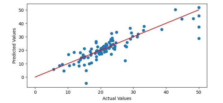
# Plot the predicted values against the actual values
plt.figure(figsize=(7.5, 3.5))
plt.scatter(y_test_sorted, y_pred[sort_idx])
plt.xlabel('Actual Values')
plt.ylabel('Predicted Values')
# Add a regression line to the plot
x = np.linspace(0, 50, 100)
y = x
plt.plot(x, y, color='red')
# Show the plot
plt.show()
Output
When you execute the program, it will produce the following plot as the output and it will print the Mean Squared Error and the Coefficient of Determination on the terminal −
Mean Squared Error: 25.215797617051855
Coefficient of Determination: 0.6903318065831567
Advertisements