Travelling Salesperson Approximation Algorithm

---

We have already discussed the travelling salesperson problem using the greedy and dynamic programming approaches, and it is established that solving the travelling salesperson problems for the perfect optimal solutions is not possible in polynomial time.

Therefore, the approximation solution is expected to find a near optimal solution for this NP-Hard problem. However, an approximate algorithm is devised only if the cost function (which is defined as the distance between two plotted points) in the problem satisfies triangle inequality.

The triangle inequality is satisfied only if the cost function c, for all the vertices of a triangle u, v and w, satisfies the following equation

                 c(u, w)≤ c(u, v)+c(v, w)

It is usually automatically satisfied in many applications.

Travelling Salesperson Approximation Algorithm

The traveling salesperson approximation algorithm requires some prerequisite algorithms to be performed so we can achieve a near optimal solution. Let us look at those prerequisite algorithms briefly −

Minimum Spanning Tree − The minimum spanning tree is a tree data structure that contains all the vertices of main graph with minimum number of edges connecting them. We apply prim’s algorithm for minimum spanning tree in this case.

Preorder Traversal − The preorder traversal is done on tree data structures where a pointer is walked through all the nodes of the tree in a [root – left child – right child] order.

Algorithm

Step 1 − Choose any vertex of the given graph randomly as the starting and ending point.

Step 2 − Construct a minimum spanning tree of the graph with the vertex chosen as the root using prim’s algorithm.

Step 3 − Once the spanning tree is constructed, preorder traversal is performed on the minimum spanning tree obtained in the previous step.

Step 4 − The preorder solution obtained is the Hamiltonian path of the travelling salesperson.

Pseudocode

APPROX_TSP(G, c)
   r <- root node of the minimum spanning tree
   T <- MST_Prim(G, c, r)
   visited = {ф}
   for i in range V:
      H <- Preorder_Traversal(G)
      visited = {H}

Analysis

The approximation algorithm of the travelling salesperson problem is a 2-approximation algorithm if the triangle inequality is satisfied.

To prove this, we need to show that the approximate cost of the problem is double the optimal cost. Few observations that support this claim would be as follows −

• The cost of minimum spanning tree is never less than the cost of the optimal Hamiltonian path. That is, c(M) ≤ c(H^*).

• The cost of full walk is also twice as the cost of minimum spanning tree. A full walk is defined as the path traced while traversing the minimum spanning tree preorderly. Full walk traverses every edge present in the graph exactly twice. Thereore, c(W) = 2c(T)

• Since the preorder walk path is less than the full walk path, the output of the algorithm is always lower than the cost of the full walk.

Example

Let us look at an example graph to visualize this approximation algorithm −

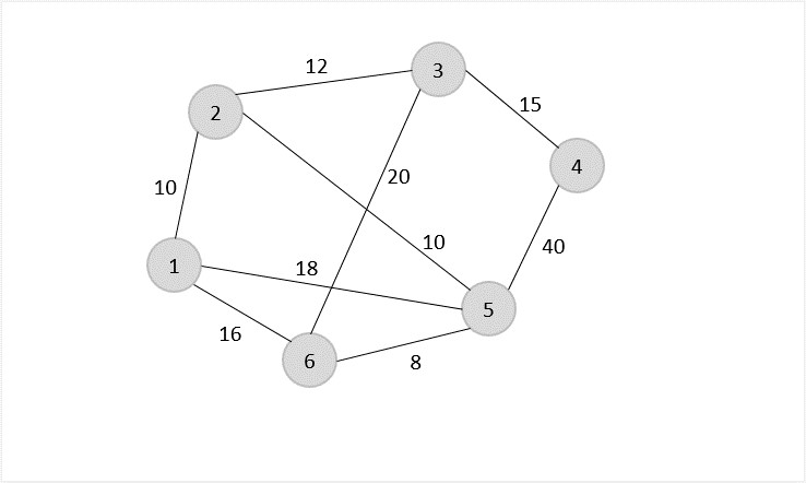
Solution

Consider vertex 1 from the above graph as the starting and ending point of the travelling salesperson and begin the algorithm from here.

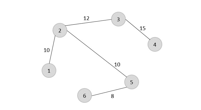
Step 1

Starting the algorithm from vertex 1, construct a minimum spanning tree from the graph. To learn more about constructing a minimum spanning tree, please click here.

Step 2

Once, the minimum spanning tree is constructed, consider the starting vertex as the root node (i.e., vertex 1) and walk through the spanning tree preorderly.

Rotating the spanning tree for easier interpretation, we get −

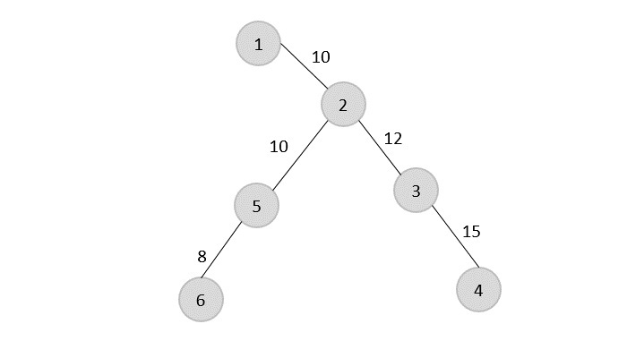
The preorder traversal of the tree is found to be − 1 → 2 → 5 → 6 → 3 → 4

Step 3

Adding the root node at the end of the traced path, we get, 1 → 2 → 5 → 6 → 3 → 4 → 1

This is the output Hamiltonian path of the travelling salesman approximation problem. The cost of the path would be the sum of all the costs in the minimum spanning tree, i.e., 55.