
Article Categories
- All Categories
-
 Data Structure
-
 Networking
-
 RDBMS
RDBMS
-
 Operating System
-
 Java
Java
-
 MS Excel
-
 iOS
iOS
-
 HTML
HTML
-
 CSS
CSS
-
 Android
-
 Python
-
 C Programming
-
 C++
C++
-
 C#
C#
-
 MongoDB
-
 MySQL
MySQL
-
 Javascript
-
 PHP
PHP
-
 Economics & Finance
TabNet in Machine Learning
In this Tutorial, we are going to learn about TabNet in Machine Learning. As far as we are aware, deep learning models have been increasingly popular for employing to solve tabular data. Due to the relevance and effectiveness of the features, they have chosen, XGBoost, RFE, and LightGBM have been dominating this stream. TabNet, however, alters the dynamic.
Researchers from Google Cloud made the TabNet proposal in 2019. The concept behind TabNet is to successfully apply deep neural networks to tabular data, which still contains a significant amount of user and processed data.
TabNet combines the best of both worlds: it is explainable (akin to simpler tree-based models) while still being fast (similar to deep neural networks). For applications in the retail, financial, and insurance sectors including forecasting, fraud detection, and credit score prediction, this makes it ideal.
Selecting the model characteristics to draw conclusions from at each stage of the model is done by TabNet using a machine learning approach called sequential attention. By using this approach, the model can learn more precise models and can explain how it generates its predictions. In addition to outperforming other neural networks and decision trees, TabNet's architecture also offers feature attributions that are easy to understand. Deep learning for tabular data is made possible by TabNet, which offers great performance and interpretability.
TabNet architecture
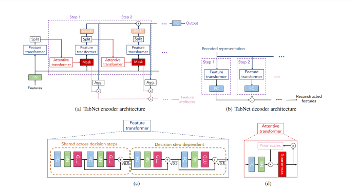
Encoder
The design, therefore, consists mostly of several consecutive stages that transmit inputs from one step to another. The report also includes some tips on how to choose the number of stages. As a result, when we take a single step, three processes occur ?
Four successive GLU decision blocks make up the feature transformer.
An attentive transformer that produces sparse feature selection using sparse-matrix facilitates interpretability and improves learning since the capacity is reserved for the most important characteristics.
The mask, together with the transformer, is used to output the decision-making parameters, n(d) and n(a), which are then passed on to the final phase.
As a result, no feature engineering has been done to the basic dataset, which includes all features. After being Batch normalized (BN), data is sent to the feature transformer where it goes through four GLU decision processes to produce two parameters.
In the case of regression or classification, the output decision n(d), which represents the prediction of continuous numbers or classes, is provided.
The next attentive transformer, where the following cycle is initiated, will receive n(a) as input.
Decoder
At the decision stage, the TabNet decoder architecture comprises a feature transformer followed by fully connected layers.
Feature Transformer
The Fully Connected Layer, Batch Normalization Layer, and GLU are the first four successive blocks in the Feature Transformer. GLU stands for the gated linear unit, which is basically the sigmoid of x multiplied by x. (GLU = ?(x) . x). Consequently, they are made up of two shared choice processes, followed by two autonomous decision phases. The layers are shared between two decision stages for robust learning since the same input characteristics are used in each phase. By guaranteeing that the variation throughout the network does not fluctuate much, normalization with a value of ?0.5 aids in stabilizing learning. It produces the two outputs n(d) and n(a), as previously explained.
Attentive Transformer
As you can see, the Attentive Transformer is made up of four layers: FC, BN, Prior Scales, and Sparsemax. Following Batch normalization, the n(a) input is sent to a fully linked layer. After that, it is multiplied by the Prior scale, a function that indicates how much you already know about the features from the preceding phases and how many features have been utilized in those steps. Every feature is equally important if it is set to 1. However, Tabnet's key benefit is that it uses soft feature selection with controlled sparsity in end-to-end learning, where one model handles both feature selection and output mapping.
Key Points to Remember
Feature, attentive, and feature masking transformers make up the TabNet encoder. A split block splits the processed representation so that it may be utilized for both the overall output and for the attentive transformer of the following phase. The feature selection mask gives interpretable data on the functionality of the model for each phase, and the masks can be combined to create a global feature significant attribution.
A feature transformer block is included in each phase of the TabNet decoder.
A feature transformer block example with a four-layer network is displayed, with two layers shared by all decision steps and the other two dependent on the decision step. Each layer is made up of BN, GLU nonlinearity, and a fully-connected (FC) layer.
An attentive transformer block illustrates this by modulating a single layer mapping using past scale data, which aggregates how much each feature was utilized before the current decision step.
TabNet Top Benefits
Encode several data kinds, such as pictures and tabular data, then solve using nonlinearity.
There is no need for Feature Engineering can toss all the columns at the model, and it will choose the best attributes that are also interpretable.
Implementing TabNet
For this tutorial, we will utilize the data from House Prices: Advanced Regression Techniques. In this example, I do not conduct any feature engineering or data cleaning, such as outlier removal, and instead, use the most basic imputation to account for any missing values.
You can download the data from here and can use it in your environment.
Installing and Importing libraries
<div class="code-mirror  language-python" contenteditable="plaintext-only" spellcheck="false" style="outline: none; overflow-wrap: break-word; overflow-y: auto; white-space: pre-wrap;">!pip install pytorch<span class="token operator">-</span>tabnet
<span class="token keyword">import</span> pandas <span class="token keyword">as</span> pd
<span class="token keyword">import</span> numpy <span class="token keyword">as</span> np
<span class="token keyword">from</span> pytorch_tabnet<span class="token punctuation">.</span>tab_model <span class="token keyword">import</span> TabNetRegressor
<span class="token keyword">from</span> sklearn<span class="token punctuation">.</span>model_selection <span class="token keyword">import</span> KFold
</div>
Dataset URL
<span class="pln">train_data_url </span><span class="pun">=</span><span class="pln"> </span><span class="str">"https://raw.githubusercontent.com/JayS420/Tabnetdataset/main/train.csv"</span><span class="pln">
test_data_url </span><span class="pun">=</span><span class="pln"> </span><span class="str">"https://raw.githubusercontent.com/JayS420/Tabnetdataset/main/test.csv"</span>
Importing Dataset
<span class="pln">train_data </span><span class="pun">=</span><span class="pln"> pd</span><span class="pun">.</span><span class="pln">read_csv</span><span class="pun">(</span><span class="pln">train_data_url</span><span class="pun">,</span><span class="pln"> error_bad_lines</span><span class="pun">=</span><span class="kwd">False</span><span class="pun">)</span><span class="pln">
test_data </span><span class="pun">=</span><span class="pln"> pd</span><span class="pun">.</span><span class="pln">read_csv</span><span class="pun">(</span><span class="pln">test_data_url</span><span class="pun">,</span><span class="pln"> error_bad_lines </span><span class="pun">=</span><span class="pln"> </span><span class="kwd">False</span><span class="pun">)</span>
Selecting some features
<div class="code-mirror  language-python" contenteditable="plaintext-only" spellcheck="false" style="outline: none; overflow-wrap: break-word; overflow-y: auto; white-space: pre-wrap;">features <span class="token operator">=</span> <span class="token punctuation">[</span><span class="token string">'LotArea'</span><span class="token punctuation">,</span> <span class="token string">'OverallQual'</span><span class="token punctuation">,</span> <span class="token string">'OverallCond'</span><span class="token punctuation">,</span> <span class="token string">'YearBuilt'</span><span class="token punctuation">,</span>
   <span class="token string">'YearRemodAdd'</span><span class="token punctuation">,</span> <span class="token string">'BsmtFinSF1'</span><span class="token punctuation">,</span> <span class="token string">'BsmtFinSF2'</span><span class="token punctuation">,</span> <span class="token string">'TotalBsmtSF'</span><span class="token punctuation">,</span>
   <span class="token string">'1stFlrSF'</span><span class="token punctuation">,</span> <span class="token string">'LowQualFinSF'</span><span class="token punctuation">,</span> <span class="token string">'GrLivArea'</span><span class="token punctuation">,</span> <span class="token string">'BsmtFullBath'</span><span class="token punctuation">,</span>
   <span class="token string">'BsmtHalfBath'</span><span class="token punctuation">,</span> <span class="token string">'HalfBath'</span><span class="token punctuation">,</span> <span class="token string">'BedroomAbvGr'</span><span class="token punctuation">,</span> <span class="token string">'Fireplaces'</span><span class="token punctuation">,</span>
   <span class="token string">'GarageCars'</span><span class="token punctuation">,</span> <span class="token string">'GarageArea'</span><span class="token punctuation">,</span> <span class="token string">'WoodDeckSF'</span><span class="token punctuation">,</span> <span class="token string">'OpenPorchSF'</span><span class="token punctuation">,</span>
   <span class="token string">'EnclosedPorch'</span><span class="token punctuation">,</span> <span class="token string">'PoolArea'</span><span class="token punctuation">,</span> <span class="token string">'YrSold'</span><span class="token punctuation">]</span>
</div>
Splitting dataset
<div class="code-mirror  language-python" contenteditable="plaintext-only" spellcheck="false" style="outline: none; overflow-wrap: break-word; overflow-y: auto; white-space: pre-wrap;">X <span class="token operator">=</span> train_data<span class="token punctuation">[</span>features<span class="token punctuation">]</span>
y <span class="token operator">=</span> np<span class="token punctuation">.</span>log1p<span class="token punctuation">(</span>train_data<span class="token punctuation">[</span><span class="token string">"SalePrice"</span><span class="token punctuation">]</span><span class="token punctuation">)</span>
X_test <span class="token operator">=</span> test_data<span class="token punctuation">[</span>features<span class="token punctuation">]</span>
y_test <span class="token operator">=</span> <span class="token punctuation">[</span><span class="token string">"SalePrice"</span><span class="token punctuation">]</span>
</div>
Filling missing data
Any missing data will be filled up with a simple mean value. Concerning the relative benefits of doing this before utilizing cross-validation.
<span class="pln">X </span><span class="pun">=</span><span class="pln"> X</span><span class="pun">.</span><span class="pln">apply</span><span class="pun">(</span><span class="kwd">lambda</span><span class="pln"> x</span><span class="pun">:</span><span class="pln"> x</span><span class="pun">.</span><span class="pln">fillna</span><span class="pun">(</span><span class="pln">x</span><span class="pun">.</span><span class="pln">mean</span><span class="pun">()),</span><span class="pln">axis</span><span class="pun">=</span><span class="lit">0</span><span class="pun">)</span><span class="pln">
X_test </span><span class="pun">=</span><span class="pln"> X_test</span><span class="pun">.</span><span class="pln">apply</span><span class="pun">(</span><span class="kwd">lambda</span><span class="pln"> x</span><span class="pun">:</span><span class="pln"> x</span><span class="pun">.</span><span class="pln">fillna</span><span class="pun">(</span><span class="pln">x</span><span class="pun">.</span><span class="pln">mean</span><span class="pun">()),</span><span class="pln">axis</span><span class="pun">=</span><span class="lit">0</span><span class="pun">)</span>
Converting data to NumPy
<div class="code-mirror  language-python" contenteditable="plaintext-only" spellcheck="false" style="outline: none; overflow-wrap: break-word; overflow-y: auto; white-space: pre-wrap;">X <span class="token operator">=</span> X<span class="token punctuation">.</span>to_numpy<span class="token punctuation">(</span><span class="token punctuation">)</span>
y <span class="token operator">=</span> y<span class="token punctuation">.</span>to_numpy<span class="token punctuation">(</span><span class="token punctuation">)</span><span class="token punctuation">.</span>reshape<span class="token punctuation">(</span><span class="token operator">-</span><span class="token number">1</span><span class="token punctuation">,</span> <span class="token number">1</span><span class="token punctuation">)</span>
X_test <span class="token operator">=</span> X_test<span class="token punctuation">.</span>to_numpy<span class="token punctuation">(</span><span class="token punctuation">)</span>
</div>
Applying Kfold validation
<div class="code-mirror  language-python" contenteditable="plaintext-only" spellcheck="false" style="outline: none; overflow-wrap: break-word; overflow-y: auto; white-space: pre-wrap;">kf <span class="token operator">=</span> KFold<span class="token punctuation">(</span>n_splits<span class="token operator">=</span><span class="token number">5</span><span class="token punctuation">,</span> random_state<span class="token operator">=</span><span class="token number">42</span><span class="token punctuation">,</span> shuffle<span class="token operator">=</span><span class="token boolean">True</span><span class="token punctuation">)</span>
predictions_array <span class="token operator">=</span><span class="token punctuation">[</span><span class="token punctuation">]</span>
CV_score_array <span class="token operator">=</span><span class="token punctuation">[</span><span class="token punctuation">]</span>
<span class="token keyword">for</span> train_index<span class="token punctuation">,</span> test_index <span class="token keyword">in</span> kf<span class="token punctuation">.</span>split<span class="token punctuation">(</span>X<span class="token punctuation">)</span><span class="token punctuation">:</span>
   X_train<span class="token punctuation">,</span> X_valid <span class="token operator">=</span> X<span class="token punctuation">[</span>train_index<span class="token punctuation">]</span><span class="token punctuation">,</span> X<span class="token punctuation">[</span>test_index<span class="token punctuation">]</span>
   y_train<span class="token punctuation">,</span> y_valid <span class="token operator">=</span> y<span class="token punctuation">[</span>train_index<span class="token punctuation">]</span><span class="token punctuation">,</span> y<span class="token punctuation">[</span>test_index<span class="token punctuation">]</span>
   regressor <span class="token operator">=</span> TabNetRegressor<span class="token punctuation">(</span>verbose<span class="token operator">=</span><span class="token number">0</span><span class="token punctuation">,</span>seed<span class="token operator">=</span><span class="token number">42</span><span class="token punctuation">)</span>
   regressor<span class="token punctuation">.</span>fit<span class="token punctuation">(</span>X_train<span class="token operator">=</span>X_train<span class="token punctuation">,</span> y_train<span class="token operator">=</span>y_train<span class="token punctuation">,</span>
      eval_set<span class="token operator">=</span><span class="token punctuation">[</span><span class="token punctuation">(</span>X_valid<span class="token punctuation">,</span> y_valid<span class="token punctuation">)</span><span class="token punctuation">]</span><span class="token punctuation">,</span>
      patience<span class="token operator">=</span><span class="token number">300</span><span class="token punctuation">,</span> max_epochs<span class="token operator">=</span><span class="token number">2000</span><span class="token punctuation">,</span>
      eval_metric<span class="token operator">=</span><span class="token punctuation">[</span><span class="token string">'rmse'</span><span class="token punctuation">]</span><span class="token punctuation">)</span>
   CV_score_array<span class="token punctuation">.</span>append<span class="token punctuation">(</span>regressor<span class="token punctuation">.</span>best_cost<span class="token punctuation">)</span>
   predictions_array<span class="token punctuation">.</span>append<span class="token punctuation">(</span>np<span class="token punctuation">.</span>expm1<span class="token punctuation">(</span>regressor<span class="token punctuation">.</span>predict<span class="token punctuation">(</span>X_test<span class="token punctuation">)</span><span class="token punctuation">)</span><span class="token punctuation">)</span>
predictions <span class="token operator">=</span> np<span class="token punctuation">.</span>mean<span class="token punctuation">(</span>predictions_array<span class="token punctuation">,</span>axis<span class="token operator">=</span><span class="token number">0</span><span class="token punctuation">)</span>
</div>
Output
Device used : cpu
Early stopping occured at epoch 1598 with best_epoch = 1298 and best_val_0_rmse
= 0.16444
Best weights from best epoch are automatically used!
Device used : cpu
Early stopping occured at epoch 1075 with best_epoch = 775 and best_val_0_rmse
= 0.12027
Best weights from best epoch are automatically used!
Device used : cpu
Early stopping occured at epoch 691 with best_epoch = 391 and best_val_0_rmse =
0.16395
Best weights from best epoch are automatically used!
Device used : cpu
Early stopping occured at epoch 679 with best_epoch = 379 and best_val_0_rmse =
0.16833
Best weights from best epoch are automatically used!
Device used : cpu
Early stopping occured at epoch 1283 with best_epoch = 983 and best_val_0_rmse
= 0.11103
Best weights from best epoch are automatically used!
Calculating Average CV score
<div class="code-mirror  language-python" contenteditable="plaintext-only" spellcheck="false" style="outline: none; overflow-wrap: break-word; overflow-y: auto; white-space: pre-wrap;"><span class="token keyword">print</span><span class="token punctuation">(</span><span class="token string">"The CV score is %.5f"</span> <span class="token operator">%</span> np<span class="token punctuation">.</span>mean<span class="token punctuation">(</span>CV_score_array<span class="token punctuation">,</span>axis<span class="token operator">=</span><span class="token number">0</span><span class="token punctuation">)</span> <span class="token punctuation">)</span>
</div>
Output
The CV score is 0.15161
Conclusion
To sum up, Tabnet is just deep learning applied to tabular data. As the learning capacity is employed for the most salient characteristics, it increases learning efficiency and enables interpretability by using sequential attention to select which features to reason from at each decision step.

2K+ Views
