- ML - Home
- ML - Introduction
- ML - Getting Started
- ML - Basic Concepts
- ML - Ecosystem
- ML - Python Libraries
- ML - Applications
- ML - Life Cycle
- ML - Required Skills
- ML - Implementation
- ML - Challenges & Common Issues
- ML - Limitations
- ML - Reallife Examples
- ML - Data Structure
- ML - Mathematics
- ML - Artificial Intelligence
- ML - Neural Networks
- ML - Deep Learning
- ML - Getting Datasets
- ML - Categorical Data
- ML - Data Loading
- ML - Data Understanding
- ML - Data Preparation
- ML - Models
- ML - Supervised Learning
- ML - Unsupervised Learning
- ML - Semi-supervised Learning
- ML - Reinforcement Learning
- ML - Supervised vs. Unsupervised
- Machine Learning Data Visualization
- ML - Data Visualization
- ML - Histograms
- ML - Density Plots
- ML - Box and Whisker Plots
- ML - Correlation Matrix Plots
- ML - Scatter Matrix Plots
- Statistics for Machine Learning
- ML - Statistics
- ML - Mean, Median, Mode
- ML - Standard Deviation
- ML - Percentiles
- ML - Data Distribution
- ML - Skewness and Kurtosis
- ML - Bias and Variance
- ML - Hypothesis
- Regression Analysis In ML
- ML - Regression Analysis
- ML - Linear Regression
- ML - Simple Linear Regression
- ML - Multiple Linear Regression
- ML - Polynomial Regression
- Classification Algorithms In ML
- ML - Classification Algorithms
- ML - Logistic Regression
- ML - K-Nearest Neighbors (KNN)
- ML - Naïve Bayes Algorithm
- ML - Decision Tree Algorithm
- ML - Support Vector Machine
- ML - Random Forest
- ML - Confusion Matrix
- ML - Stochastic Gradient Descent
- Clustering Algorithms In ML
- ML - Clustering Algorithms
- ML - Centroid-Based Clustering
- ML - K-Means Clustering
- ML - K-Medoids Clustering
- ML - Mean-Shift Clustering
- ML - Hierarchical Clustering
- ML - Density-Based Clustering
- ML - DBSCAN Clustering
- ML - OPTICS Clustering
- ML - HDBSCAN Clustering
- ML - BIRCH Clustering
- ML - Affinity Propagation
- ML - Distribution-Based Clustering
- ML - Agglomerative Clustering
- Dimensionality Reduction In ML
- ML - Dimensionality Reduction
- ML - Feature Selection
- ML - Feature Extraction
- ML - Backward Elimination
- ML - Forward Feature Construction
- ML - High Correlation Filter
- ML - Low Variance Filter
- ML - Missing Values Ratio
- ML - Principal Component Analysis
- Reinforcement Learning
- ML - Reinforcement Learning Algorithms
- ML - Exploitation & Exploration
- ML - Q-Learning
- ML - REINFORCE Algorithm
- ML - SARSA Reinforcement Learning
- ML - Actor-critic Method
- ML - Monte Carlo Methods
- ML - Temporal Difference
- Deep Reinforcement Learning
- ML - Deep Reinforcement Learning
- ML - Deep Reinforcement Learning Algorithms
- ML - Deep Q-Networks
- ML - Deep Deterministic Policy Gradient
- ML - Trust Region Methods
- Quantum Machine Learning
- ML - Quantum Machine Learning
- ML - Quantum Machine Learning with Python
- Machine Learning Miscellaneous
- ML - Performance Metrics
- ML - Automatic Workflows
- ML - Boost Model Performance
- ML - Gradient Boosting
- ML - Bootstrap Aggregation (Bagging)
- ML - Cross Validation
- ML - AUC-ROC Curve
- ML - Grid Search
- ML - Data Scaling
- ML - Train and Test
- ML - Association Rules
- ML - Apriori Algorithm
- ML - Gaussian Discriminant Analysis
- ML - Cost Function
- ML - Bayes Theorem
- ML - Precision and Recall
- ML - Adversarial
- ML - Stacking
- ML - Epoch
- ML - Perceptron
- ML - Regularization
- ML - Overfitting
- ML - P-value
- ML - Entropy
- ML - MLOps
- ML - Data Leakage
- ML - Monetizing Machine Learning
- ML - Types of Data
- Machine Learning - Resources
- ML - Quick Guide
- ML - Cheatsheet
- ML - Interview Questions
- ML - Useful Resources
- ML - Discussion
Clustering Algorithms in Machine Learning
Clustering Algorithms are one of the most useful unsupervised machine learning methods. These methods are used to find similarity as well as the relationship patterns among data samples and then cluster those samples into groups having similarity based on features.
Clustering is important because it determines the intrinsic grouping among the present unlabeled data. They basically make some assumptions about data points to constitute their similarity. Each assumption will construct different but equally valid clusters.
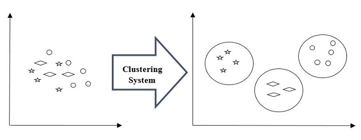
For example, below is the diagram which shows clustering system grouped together the similar kind of data in different clusters −
Cluster Formation Methods
It is not necessary that clusters will be formed in spherical form. Followings are some other cluster formation methods −
Density-based
In these methods, the clusters are formed as the dense region. The advantage of these methods is that they have good accuracy as well as good ability to merge two clusters. Ex. Density-Based Spatial Clustering of Applications with Noise (DBSCAN), Ordering Points to identify Clustering structure (OPTICS) etc.
Hierarchical-based
In these methods, the clusters are formed as a tree type structure based on the hierarchy. They have two categories namely, Agglomerative (Bottom up approach) and Divisive (Top down approach). Ex. Clustering using Representatives (CURE), Balanced iterative Reducing Clustering using Hierarchies (BIRCH) etc.
Partitioning
In these methods, the clusters are formed by portioning the objects into k clusters. Number of clusters will be equal to the number of partitions. Ex. K-means, Clustering Large Applications based upon randomized Search (CLARANS).
Grid
In these methods, the clusters are formed as a grid like structure. The advantage of these methods is that all the clustering operation done on these grids are fast and independent of the number of data objects. Ex. Statistical Information Grid (STING), Clustering in Quest (CLIQUE).
Clustering Algorithms in Machine Learning
The following are the most important and useful machine learning clustering algorithms −
- K-Means Clustering
- K-Medoids Clustering
- Mean-Shift Clustering
- DBSCAN Clustering
- OPTICS Clustering
- HDBSCAN Clustering
- BIRCH algorithm
- Affinity Propagation Clustering
- Agglomerative Clustering
- Gaussian Mixture Model
K-Means Clustering
The K-Means clustering algorithm computes the centroids and iterates until we it finds optimal centroid. It assumes that the number of clusters are already known. It is also called flat clustering algorithm. The number of clusters identified from data by algorithm is represented by 'K' in K-means.
K-Medoids Clustering
The K-Methoids Clustering is an improved version of K-means clustering algorithm. Working is as follows
- Select k random data points from the dataset as the initial medoids.
- Assign each data point to the nearest medoid.
- For each cluster, select the data point that minimizes the sum of distances to all the other data points in the cluster, and set it as the new medoid.
- Repeat steps 2 and 3 until convergence or a maximum number of iterations is reached.
Mean-Shift Clustering
Mean-Shift ClusteringIt is another powerful clustering algorithm used in unsupervised learning. Unlike K-means clustering, it does not make any assumptions hence it is a non-parametric algorithm.
DBSCAN Clustering
The DBSCAN (Density-Based Spatial Clustering of Applications with Noise) algorithm is one of the most common density-based clustering algorithms. The DBSCAN algorithm requires two parameters: the minimum number of neighbors (minPts) and the maximum distance between core data points (eps).
OPTICS Clustering
OPTICS (Ordering Points to Identify the Clustering Structure) is like DBSCAN, another popular density-based clustering algorithm. However, OPTICS has several advantages over DBSCAN, including the ability to identify clusters of varying densities, the ability to handle noise, and the ability to produce a hierarchical clustering structure.
HDBSCAN Clustering
HDBSCAN (Hierarchical Density-Based Spatial Clustering of Applications with Noise) is a clustering algorithm that is based on density clustering. It is a newer algorithm that builds upon the popular DBSCAN algorithm and offers several advantages over it, such as better handling of clusters of varying densities and the ability to detect clusters of different shapes and sizes.
BIRCH algorithm
BIRCH (Balanced Iterative Reducing and Clustering hierarchies) is a hierarchical clustering algorithm that is designed to handle large datasets efficiently. The algorithm builds a treelike structure of clusters by recursively partitioning the data into subclusters until a stopping criterion is met.
Affinity Propagation Clustering
Affinity Propagation is a clustering algorithm that identifies "exemplars" in a dataset and assigns each data point to one of these exemplars. It is a type of clustering algorithm that does not require a pre-specified number of clusters, making it a useful tool for exploratory data analysis. Affinity Propagation was introduced by Frey and Dueck in 2007 and has since been widely used in many fields such as biology, computer vision, and social network analysis.
Agglomerative Clustering
Agglomerative clustering is a hierarchical clustering algorithm that starts with each data point as its own cluster and iteratively merges the closest clusters until a stopping criterion is reached. It is a bottom-up approach that produces a dendrogram, which is a tree-like diagram that shows the hierarchical relationship between the clusters. The algorithm can be implemented using the scikit-learn library in Python.
Gaussian Mixture Model
Gaussian Mixture Models (GMM) is a popular clustering algorithm used in machine learning that assumes that the data is generated from a mixture of Gaussian distributions. In other words, GMM tries to fit a set of Gaussian distributions to the data, where each Gaussian distribution represents a cluster in the data.
Measuring Clustering Performance
One of the most important consideration regarding ML model is assessing its performance or you can say model's quality. In case of supervised learning algorithms, assessing the quality of our model is easy because we already have labels for every example.
On the other hand, in case of unsupervised learning algorithms we are not that much blessed because we deal with unlabeled data. But still we have some metrics that give the practitioner an insight about the happening of change in clusters depending on algorithm.
Before we deep dive into such metrics, we must understand that these metrics only evaluates the comparative performance of models against each other rather than measuring the validity of the model's prediction. Followings are some of the metrics that we can deploy on clustering algorithms to measure the quality of model −
1. Silhouette Analysis 2. Davis-Bouldin Index 3. Dunn Index1. Silhouette Analysis
Silhouette analysis used to check the quality of clustering model by measuring the distance between the clusters. It basically provides us a way to assess the parameters like number of clusters with the help of Silhouette score. This score measures how close each point in one cluster is to points in the neighboring clusters.
Analysis of Silhouette Score
The range of Silhouette score is [-1, 1]. Its analysis is as follows −
+1 Score − Near +1 Silhouette score indicates that the sample is far away from its neighboring cluster.
0 Score − 0 Silhouette score indicates that the sample is on or very close to the decision boundary separating two neighboring clusters.
-1 Score &minusl -1 Silhouette score indicates that the samples have been assigned to the wrong clusters.
The calculation of Silhouette score can be done by using the following formula −
=()/ (,)
Here, = mean distance to the points in the nearest cluster
And, = mean intra-cluster distance to all the points.
2. Davis-Bouldin Index
DB index is another good metric to perform the analysis of clustering algorithms. With the help of DB index, we can understand the following points about clustering model −
Weather the clusters are well-spaced from each other or not?
How much dense the clusters are?
We can calculate DB index with the help of following formula −
$$DB=\frac{1}{n}\displaystyle\sum\limits_{i=1}^n max_{j\neq{i}}\left(\frac{\sigma_{i}+\sigma_{j}}{d(c_{i},c_{j})}\right)$$Here, = number of clusters
σi = average distance of all points in cluster from the cluster centroid .
Less the DB index, better the clustering model is.
3. Dunn Index
It works same as DB index but there are following points in which both differs −
The Dunn index considers only the worst case i.e. the clusters that are close together while DB index considers dispersion and separation of all the clusters in clustering model.
Dunn index increases as the performance increases while DB index gets better when clusters are well-spaced and dense.
We can calculate Dunn index with the help of following formula −
$$D=\frac{min_{1\leq i <{j}\leq{n}}P(i,j)}{mix_{1\leq i < k \leq n}q(k)}$$Here, ,, = each indices for clusters
= inter-cluster distance
q = intra-cluster distance
Applications of Clustering
We can find clustering useful in the following areas −
Data summarization and compression − Clustering is widely used in the areas where we require data summarization, compression and reduction as well. The examples are image processing and vector quantization.
Collaborative systems and customer segmentation − Since clustering can be used to find similar products or same kind of users, it can be used in the area of collaborative systems and customer segmentation.
Serve as a key intermediate step for other data mining tasks − Cluster analysis can generate a compact summary of data for classification, testing, hypothesis generation; hence, it serves as a key intermediate step for other data mining tasks also.
Trend detection in dynamic data − Clustering can also be used for trend detection in dynamic data by making various clusters of similar trends.
Social network analysis − Clustering can be used in social network analysis. The examples are generating sequences in images, videos or audios.
Biological data analysis − Clustering can also be used to make clusters of images, videos hence it can successfully be used in biological data analysis.
