- Artificial Neural Network - Home
- Basic Concepts
- Building Blocks
- Learning & Adaptation
- Supervised Learning
- Unsupervised Learning
- Learning Vector Quantization
- Adaptive Resonance Theory
- Kohonen Self-Organizing Feature Maps
- Associate Memory Network
- Hopfield Networks
- Boltzmann Machine
- Brain-State-in-a-Box Network
- Optimization Using Hopfield Network
- Other Optimization Techniques
- Genetic Algorithm
- Applications of Neural Networks
Unsupervised Neural Networks
As the name suggests, this type of learning is done without the supervision of a teacher. This learning process is independent. During the training of ANN under unsupervised learning, the input vectors of similar type are combined to form clusters. When a new input pattern is applied, then the neural network gives an output response indicating the class to which input pattern belongs. In this, there would be no feedback from the environment as to what should be the desired output and whether it is correct or incorrect. Hence, in this type of learning the network itself must discover the patterns, features from the input data and the relation for the input data over the output.
Winner-Takes-All Networks
These kinds of networks are based on the competitive learning rule and will use the strategy where it chooses the neuron with the greatest total inputs as a winner. The connections between the output neurons show the competition between them and one of them would be ON which means it would be the winner and others would be OFF.
Following are some of the networks based on this simple concept using unsupervised learning.
Hamming Network
In most of the neural networks using unsupervised learning, it is essential to compute the distance and perform comparisons. This kind of network is Hamming network, where for every given input vectors, it would be clustered into different groups. Following are some important features of Hamming Networks −
Lippmann started working on Hamming networks in 1987.
It is a single layer network.
The inputs can be either binary {0, 1} of bipolar {-1, 1}.
The weights of the net are calculated by the exemplar vectors.
It is a fixed weight network which means the weights would remain the same even during training.
Max Net
This is also a fixed weight network, which serves as a subnet for selecting the node having the highest input. All the nodes are fully interconnected and there exists symmetrical weights in all these weighted interconnections.
Architecture
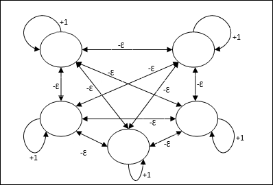
It uses the mechanism which is an iterative process and each node receives inhibitory inputs from all other nodes through connections. The single node whose value is maximum would be active or winner and the activations of all other nodes would be inactive. Max Net uses identity activation function with $$f(x)\:=\:\begin{cases}x & if\:x > 0\\0 & if\:x \leq 0\end{cases}$$
The task of this net is accomplished by the self-excitation weight of +1 and mutual inhibition magnitude, which is set like [0 < ɛ < $\frac{1}{m}$] where m is the total number of the nodes.
Competitive Learning in ANN
It is concerned with unsupervised training in which the output nodes try to compete with each other to represent the input pattern. To understand this learning rule we will have to understand competitive net which is explained as follows −
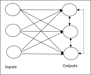
Basic Concept of Competitive Network
This network is just like a single layer feed-forward network having feedback connection between the outputs. The connections between the outputs are inhibitory type, which is shown by dotted lines, which means the competitors never support themselves.
Basic Concept of Competitive Learning Rule
As said earlier, there would be competition among the output nodes so the main concept is - during training, the output unit that has the highest activation to a given input pattern, will be declared the winner. This rule is also called Winner-takes-all because only the winning neuron is updated and the rest of the neurons are left unchanged.
Mathematical Formulation
Following are the three important factors for mathematical formulation of this learning rule −
Condition to be a winner
Suppose if a neuron yk wants to be the winner, then there would be the following condition
$$y_{k}\:=\:\begin{cases}1 & if\:v_{k} > v_{j}\:for\:all\:\:j,\:j\:\neq\:k\\0 & otherwise\end{cases}$$
It means that if any neuron, say, yk wants to win, then its induced local field (the output of the summation unit), say vk, must be the largest among all the other neurons in the network.
Condition of the sum total of weight
Another constraint over the competitive learning rule is the sum total of weights to a particular output neuron is going to be 1. For example, if we consider neuron k then
$$\displaystyle\sum\limits_{k} w_{kj}\:=\:1\:\:\:\:for\:all\:\:k$$
Change of weight for the winner
If a neuron does not respond to the input pattern, then no learning takes place in that neuron. However, if a particular neuron wins, then the corresponding weights are adjusted as follows −
$$\Delta w_{kj}\:=\:\begin{cases}-\alpha(x_{j}\:-\:w_{kj}), & if\:neuron\:k\:wins\\0 & if\:neuron\:k\:losses\end{cases}$$
Here $\alpha$ is the learning rate.
This clearly shows that we are favoring the winning neuron by adjusting its weight and if a neuron is lost, then we need not bother to re-adjust its weight.
K-means Clustering Algorithm
K-means is one of the most popular clustering algorithm in which we use the concept of partition procedure. We start with an initial partition and repeatedly move patterns from one cluster to another, until we get a satisfactory result.
Algorithm
Step 1 − Select k points as the initial centroids. Initialize k prototypes (w1,,wk), for example we can identifying them with randomly chosen input vectors −
$$W_{j}\:=\:i_{p},\:\:\: where\:j\:\in \lbrace1,....,k\rbrace\:and\:p\:\in \lbrace1,....,n\rbrace$$
Each cluster Cj is associated with prototype wj.
Step 2 − Repeat step 3-5 until E no longer decreases, or the cluster membership no longer changes.
Step 3 − For each input vector ip where p ∈ {1,,n}, put ip in the cluster Cj* with the nearest prototype wj* having the following relation
$$|i_{p}\:-\:w_{j*}|\:\leq\:|i_{p}\:-\:w_{j}|,\:j\:\in \lbrace1,....,k\rbrace$$
Step 4 − For each cluster Cj, where j ∈ { 1,,k}, update the prototype wj to be the centroid of all samples currently in Cj , so that
$$w_{j}\:=\:\sum_{i_{p}\in C_{j}}\frac{i_{p}}{|C_{j}|}$$
Step 5 − Compute the total quantization error as follows −
$$E\:=\:\sum_{j=1}^k\sum_{i_{p}\in w_{j}}|i_{p}\:-\:w_{j}|^2$$
Neocognitron
It is a multilayer feedforward network, which was developed by Fukushima in 1980s. This model is based on supervised learning and is used for visual pattern recognition, mainly hand-written characters. It is basically an extension of Cognitron network, which was also developed by Fukushima in 1975.
Architecture
It is a hierarchical network, which comprises many layers and there is a pattern of connectivity locally in those layers.
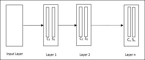
As we have seen in the above diagram, neocognitron is divided into different connected layers and each layer has two cells. Explanation of these cells is as follows −
S-Cell − It is called a simple cell, which is trained to respond to a particular pattern or a group of patterns.
C-Cell − It is called a complex cell, which combines the output from S-cell and simultaneously lessens the number of units in each array. In another sense, C-cell displaces the result of S-cell.
Training Algorithm
Training of neocognitron is found to be progressed layer by layer. The weights from the input layer to the first layer are trained and frozen. Then, the weights from the first layer to the second layer are trained, and so on. The internal calculations between S-cell and Ccell depend upon the weights coming from the previous layers. Hence, we can say that the training algorithm depends upon the calculations on S-cell and C-cell.
Calculations in S-cell
The S-cell possesses the excitatory signal received from the previous layer and possesses inhibitory signals obtained within the same layer.
$$\theta=\:\sqrt{\sum\sum t_{i} c_{i}^2}$$
Here, ti is the fixed weight and ci is the output from C-cell.
The scaled input of S-cell can be calculated as follows −
$$x\:=\:\frac{1\:+\:e}{1\:+\:vw_{0}}\:-\:1$$
Here, $e\:=\:\sum_i c_{i}w_{i}$
wi is the weight adjusted from C-cell to S-cell.
w0 is the weight adjustable between the input and S-cell.
v is the excitatory input from C-cell.
The activation of the output signal is,
$$s\:=\:\begin{cases}x, & if\:x \geq 0\\0, & if\:x
Calculations in C-cell
The net input of C-layer is
$$C\:=\:\displaystyle\sum\limits_i s_{i}x_{i}$$
Here, si is the output from S-cell and xi is the fixed weight from S-cell to C-cell.
The final output is as follows −
$$C_{out}\:=\:\begin{cases}\frac{C}{a+C}, & if\:C > 0\\0, & otherwise\end{cases}$$
Here a is the parameter that depends on the performance of the network.
