
Article Categories
- All Categories
-
 Data Structure
-
 Networking
-
 RDBMS
RDBMS
-
 Operating System
-
 Java
Java
-
 MS Excel
-
 iOS
iOS
-
 HTML
HTML
-
 CSS
CSS
-
 Android
-
 Python
-
 C Programming
-
 C++
C++
-
 C#
C#
-
 MongoDB
-
 MySQL
MySQL
-
 Javascript
-
 PHP
PHP
-
 Economics & Finance
How to lookup to return an active hyperlink in excel?
In Excel, performing a lookup to return an active hyperlink can be a useful technique when you want to dynamically generate clickable links based on specific values. Although Excel does not have a direct function for this purpose, you can combine the VLOOKUP or INDEX function with the HYPERLINK function to achieve the desired result. This combination allows you to search for a value, retrieve a corresponding URL or address, and create an active hyperlink that can be clicked to navigate to the associated location.
In this article will consider one simple example to learn the process of obtaining an active hyperlink by using the look-up return.
Example 1: To look up the active hyperlink in excel by using the user defined formula
Step 1
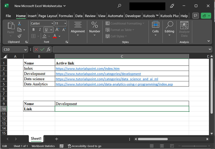
To understand the process of extracting active hyperlinks from an excel sheet. Consider the below provided excel sheet. This excels sheet contains two columns. Here first column contains relevant name information for hyperlink. While the second column contains data for active link. After that go to the B9 cell and type the name as "Development". Further, go to the B10 cell and type the column header as "link". Make cell C10 empty. This cell will hold the relevant hyperlink. Cell C9 contains name information for required hyperlink.
Step 2
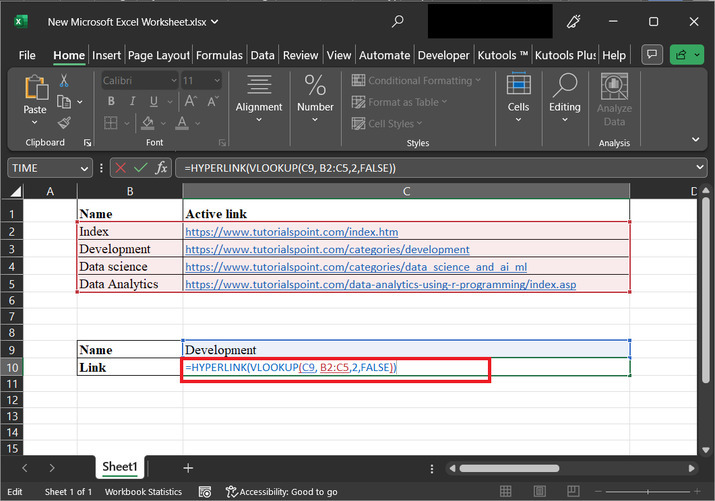
Go to the C10, cell, and type the formula "=HYPERLINK(VLOOKUP(C9, B2:C5,2,FALSE))". Snapshot for the same is provided below ?
Explanation for formula
VLOOKUP (C9, B2:C5, 2, FALSE) ? It is used to retrieve a value presented in the B column of a range (B2:C5) and return a resulting value from the C column of that range. In this case, it looks for the value in cell C9. The "2" as the fourth argument indicates that the function would retrieve the value from the C column of the range. The "FALSE" at the end indicates that an exact match is required.
HYPERLINK (VLOOKUP (C9, B2:C5, 2, FALSE)) ? The result of the previous function that is VLOOKUP would be passed as an argument to this function which is essential to create the hyperlink with a clickable link in Excel. In this case, the result of the VLOOKUP function is used as the URL or address for the hyperlink.
Step 3
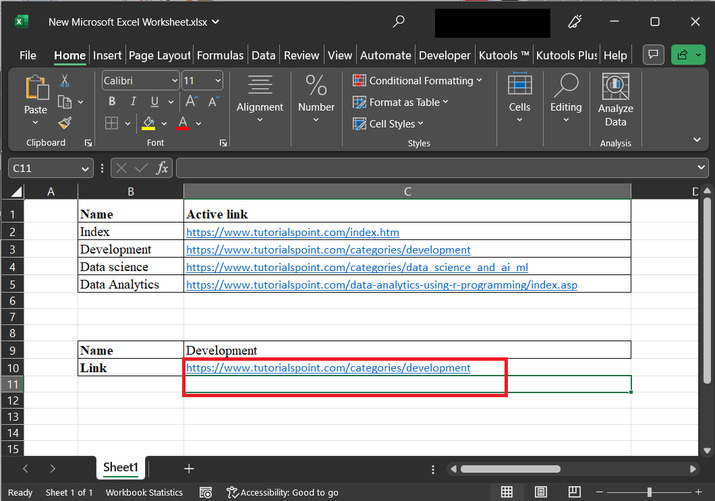
Finally, press "Enter" key to obtain the required result.
Conclusion
By leveraging the power of Excel functions, such as VLOOKUP or INDEX, along with the HYPERLINK function, the user can efficiently perform lookups to return active hyperlinks in Excel. This enables users to create dynamic and interactive spreadsheets where users can easily navigate to relevant web pages or file locations by simply clicking on the generated hyperlinks. Using this approach, users can enhance the usability and functionality of Excel workbooks, making them more intuitive and user-friendly.

7K+ Views
