
Article Categories
- All Categories
-
 Data Structure
-
 Networking
-
 RDBMS
RDBMS
-
 Operating System
-
 Java
Java
-
 MS Excel
-
 iOS
iOS
-
 HTML
HTML
-
 CSS
CSS
-
 Android
-
 Python
-
 C Programming
-
 C++
C++
-
 C#
C#
-
 MongoDB
-
 MySQL
MySQL
-
 Javascript
-
 PHP
PHP
-
 Economics & Finance
How To Do Three-Way Lookup In Excel?
Excel is a strong tool for organising and analysing data, and knowing how to execute a three?way lookup will considerably improve your data analysis skills. A three?way lookup is a mechanism for retrieving data from a table based on three distinct criteria. This is especially handy if you have a large dataset with several variables and need to identify a single value that meets three criteria.
In this article, we will show you how to execute a three?way lookup in Excel step by step. We'll go over different ways and functions for completing this task, including as the INDEX?MATCH?MATCH formula and the VLOOKUP formula combined with auxiliary columns. Mastering the technique of three?way lookups will allow you to rapidly navigate complex databases and extract the information you require, whether you are a data analyst, a business professional, or a student. So, let's get started and look at how to execute three?way lookups in Excel!
Do Three?Way Lookup
Here we will use the formula directly to complete the task. So let us see a simple process to learn how you can do a three?way lookup in Excel.
Step 1
Consider an Excel sheet where the data in the sheet is similar to the below image.
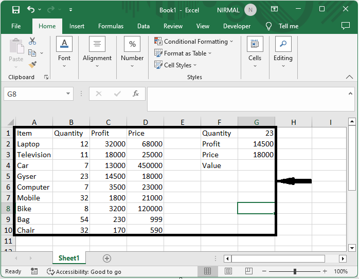
First, click on an empty cell, in our case, cell G4, and enter the formula as =INDEX($A$2:$D$10,MATCH(G1&G2,$A$2:$A$10&$B$2:$B$10,0), MATCH(G3,$A$1:$D1,0)) and click Ctrl + Shift + Enter to complete the task.
Empty cell > Formula > Ctrl + Shift + Enter.
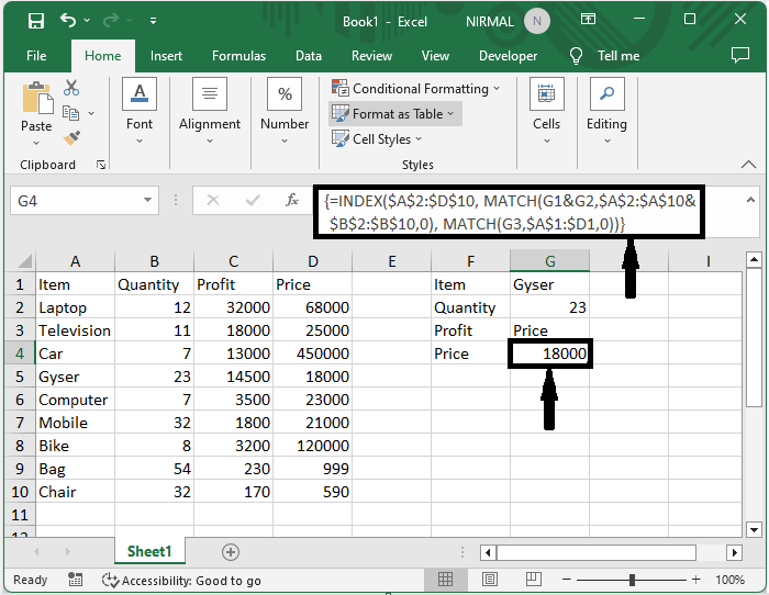
Formula division
$A$2:$D$10: The range of cells.
G1 and G2: Criteria 1 and Criteria 2.
$A$2:$A$10 &$B$2:$B$11: Two ranges that criteria 1 and criteria 2 are in.
G3, $A$1: $D$1: Criteria 3, and the range that criteria 3 is in.
Conclusion
In this tutorial, we have used a simple example to demonstrate how you can do a three?way lookup in Excel to highlight a particular set of data.

5K+ Views
