- Excel Charts - Home
- Excel Charts - Introduction
- Excel Charts - Creating Charts
- Excel Charts - Types
- Excel Charts - Column Chart
- Excel Charts - Line Chart
- Excel Charts - Pie Chart
- Excel Charts - Doughnut Chart
- Excel Charts - Bar Chart
- Excel Charts - Area Chart
- Excel Charts - Scatter (X Y) Chart
- Excel Charts - Bubble Chart
- Excel Charts - Stock Chart
- Excel Charts - Surface Chart
- Excel Charts - Radar Chart
- Excel Charts - Combo Chart
- Excel Charts - Chart Elements
- Excel Charts - Chart Styles
- Excel Charts - Chart Filters
- Excel Charts - Fine Tuning
- Excel Charts - Design Tools
- Excel Charts - Quick Formatting
- Excel Charts - Aesthetic Data Labels
- Excel Charts - Format Tools
- Excel Charts - Sparklines
- Excel Charts - PivotCharts
Excel Charts - Stock Chart
Stock charts, as the name indicates are useful to show fluctuations in stock prices. However, these charts are useful to show fluctuations in other data also, such as daily rainfall or annual temperatures.
If you use a Stock chart to display the fluctuation of stock prices, you can also incorporate the trading volume.
For Stock charts, the data needs to be in a specific order. For example, to create a simple high-low-close Stock chart, arrange your data with high, low, and close entered as column headings, in that order.
Follow the steps given below to insert a Stock chart in your worksheet.
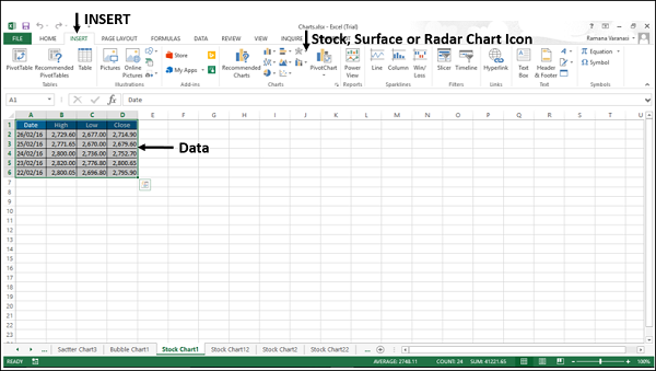
Step 1 − Arrange the data in columns or rows on the worksheet.
Step 2 − Select the data.
Step 3 − On the INSERT tab, in the Charts group, click the Stock, Surface or Radar chart icon on the Ribbon.
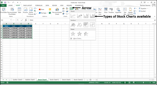
You will see the different types of available Stock charts.
A Stock chart has the following sub-types −
- High-Low-Close
- Open-High-Low-Close
- Volume-High-Low-Close
- Volume-Open-High-Low-Close
In this chapter, you will understand when each of the Stock chart types is useful.
High-Low-Close
The High-Low-Close Stock chart is often used to illustrate the stock prices. It requires three series of values in the following order- High, Low, and then Close.
To create this chart, arrange the data in the Order - High, Low, and Close.
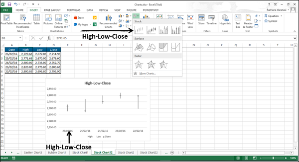
You can use the High-Low-Close Stock chart to show the trend of stocks over a period of time.
Open-High-Low-Close
The Open-High-Low-Close Stock chart is also used to illustrate the stock prices. It requires four series of values in the following order: Open, High, Low, and then Close.
To create this chart, arrange the data in the order - Open, High, Low, and Close.
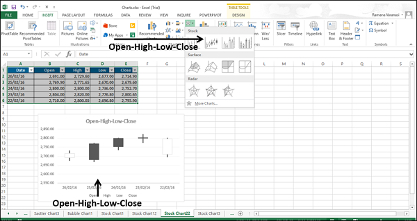
You can use the Open-High-Low-Close Stock chart to show the trend of STOCKS over a period of time.
Volume-High-Low-Close
The Volume-High-Low-Close Stock chart is also used to illustrate the stock prices. It requires four series of values in the following order: Volume, High, Low, and then Close.
To create this chart, arrange the data in the order − Volume, High, Low, and Close.
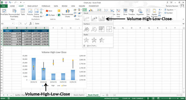
You can use the Volume-High-Low-Close Stock Chart to show the trend of stocks over a period of time.
Volume-Open-High-Low-Close
The Volume-Open-High-Low-Close Stock chart is also used to illustrate the stock prices. It requires five series of values in the following order: Volume, Open, High, Low, and then Close.
To create this chart, arrange the data in the order - Volume, Open, High, Low, and Close.
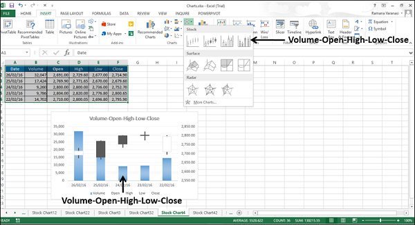
You can use the Volume-Open-High-Low-Close Stock chart to show the trend of stocks over a period of time.
