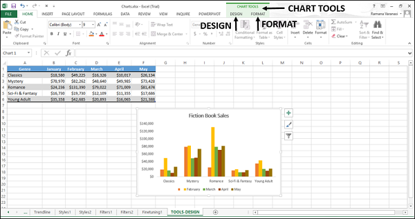
Excel Charts - Design Tools

---

Chart tools comprise of two tabs DESIGN and FORMAT.

Step 1 − When you click on a chart, CHART TOOLS comprising of DESIGN and FORMAT tabs appear on the Ribbon.

Step 2 − Click the DESIGN tab on the Ribbon. The Ribbon changes to the DESIGN commands.

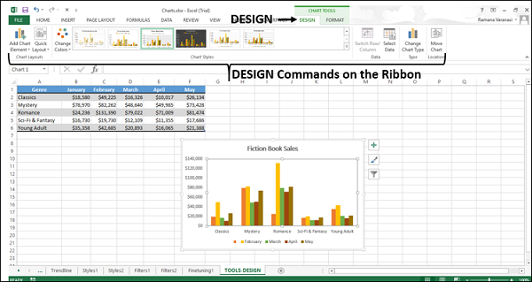
The Ribbon contains the following Design commands −

• Chart layouts group

  • Add chart element

  • Quick layout

• Chart styles group

  • Change colors

  • Chart styles

• Data group

  • Switch row/column

  • Select data

• Type group

  • Change chart type

• Location group

  • Move chart

In this chapter, you will understand the design commands on the Ribbon.

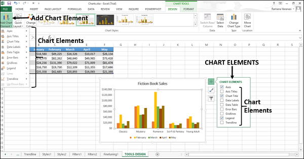
Add Chart Element

Add Chart Element is the same as chart elements.

Step 1 − Click Add Chart Element. The chart elements appear in the drop-down list. These are same as those in the chart elements list.

Refer to the chapter – Chart Elements in this tutorial.

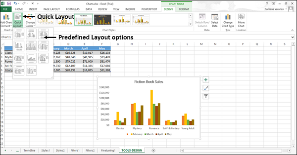
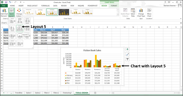
Quick Layout

You can use Quick Layout to change the overall layout of the chart quickly by choosing one of the predefined layout options.

Step 1 − On the Ribbon, click Quick Layout. Different predefined layout options will be displayed.

Step 2 − Move the pointer across the predefined layout options. The chart layout changes dynamically to the particular option.

Step 3 − Select the layout you want. The chart will be displayed with the chosen layout.

Change Colors

The functions of Change Colors are the same as Chart Styles → COLOR.

Step 1 − On the Ribbon, click Change Colors. The color schemes appear in the drop-down list. These are the same as that appear in Change Styles → COLOR.

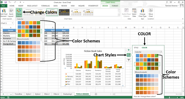
Refer to the chapter – Chart Styles in this tutorial.

Chart Styles

The Chart Styles command is the same as Chart Styles → STYLE.

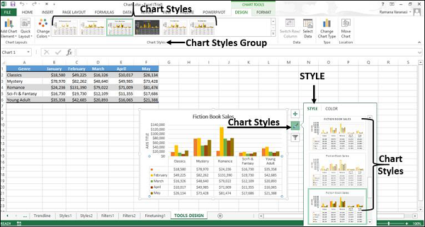
Refer to the chapter – Chart Styles in this tutorial.

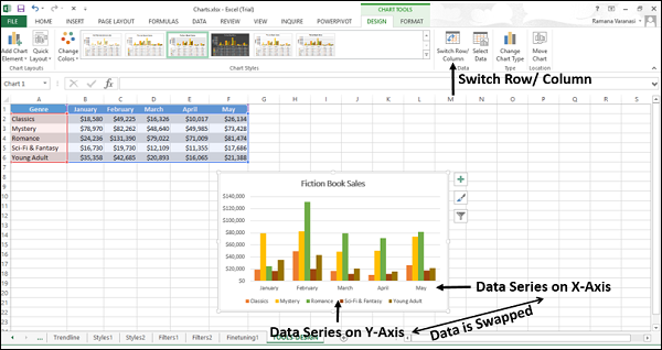
Switch Row/Column

You can use Switch Row/Column to change the data being displayed on X-axis to be displayed on Y-axis and vice versa.

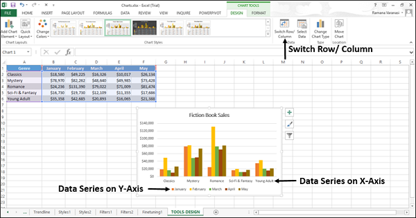
Click Switch Row / Column. The data will be swapped between X-axis and Y-axis on the chart.

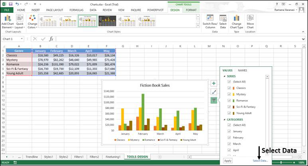
Select Data

You can use Select Data to change the data range included in the chart.

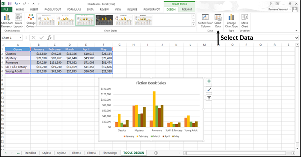
Step 1 − Click Select Data. A Select Data Source window appears.

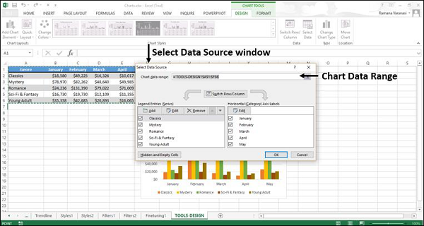
This window is the same as that appears with Chart Styles → Select data.

Step 2 − Select the chart data range in the select data source window.

Step 3 − Select the data that you want to display on your chart form the Excel worksheet.

Change Chart Type

You can use the Change Chart Type button to change your chart to a different chart type.

Step 1 − Click Change Chart Type. A Change Chart Type window appears.

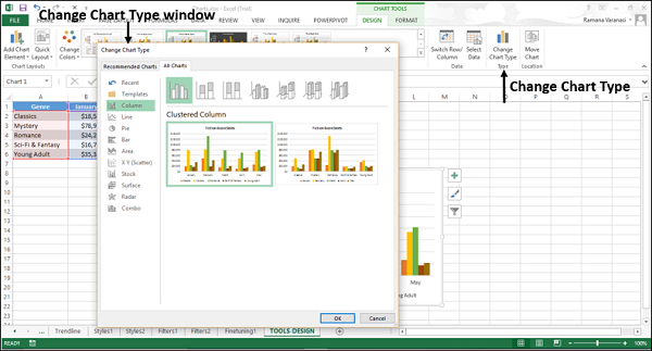
Step 2 − Select the chart type you want.

Your chart will be displayed with the chart type you want.

Move Chart

You can use Move Chart to move the chart to another worksheet in the workbook.

Step 1 − Click the Move Chart command button. A Move Chart window appears.

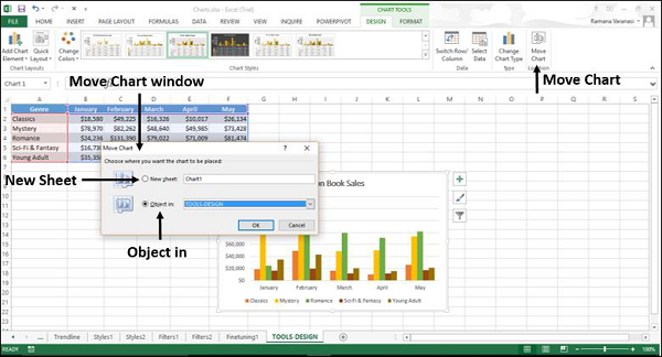
Step 2 − Select New Sheet. Type the name of the new sheet.

The chart moves from the existing sheet to the new sheet.