Excel Charts - Creating Charts

---

---

In this chapter, we will learn to create charts.

Creating Charts with Insert Chart

To create charts using the Insert Chart tab, follow the steps given below.

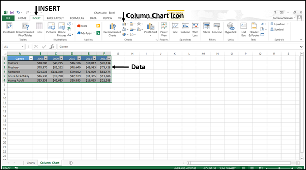
Step 1 − Select the data.

Step 2 − Click the Insert tab on the Ribbon.

Step 3 − Click the Insert Column Chart on the Ribbon.

The 2-D column, 3-D Column chart options are displayed. Further, More Column Charts… option is also displayed.

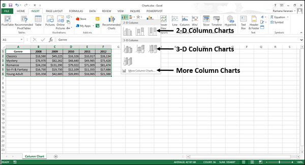
Step 4 − Move through the Column Chart options to see the previews.

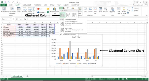
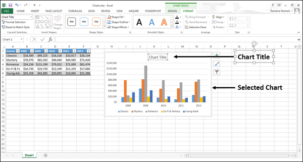
Step 5 − Click Clustered Column. The chart will be displayed in your worksheet.

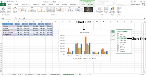
Step 6 − Give a meaningful title to the chart by editing Chart Title.

Creating Charts with Recommended Charts

You can use the Recommended Charts option if −

• You want to create a chart quickly.

• You are not sure of the chart type that suits your data.

• If the chart type you selected is not working with your data.

To use the option Recommended Charts, follow the steps given below −

Step 1 − Select the data.

Step 2 − Click the Insert tab on the Ribbon.

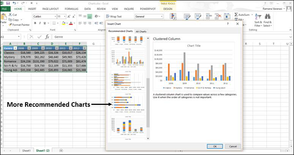
Step 3 − Click Recommended Charts.

A window displaying the charts that suit your data will be displayed, under the tab Recommended Charts.

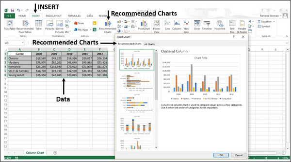
Step 4 − Browse through the Recommended Charts.

Step 5 − Click on a chart type to see the preview on the right side.

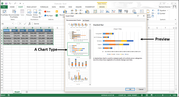
Step 6 − Select the chart type you like. Click OK. The chart will be displayed in your worksheet.

If you do not see a chart you like, click the All Charts tab to see all the available chart types and pick a chart.

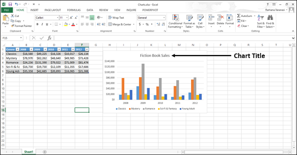
Step 7 − Give a meaningful title to the chart by editing Chart Title.

Creating Charts with Quick Analysis

Follow the steps given to create a chart with Quick Analysis.

Step 1 − Select the data.

A Quick Analysis button appears at the bottom right of your selected data.

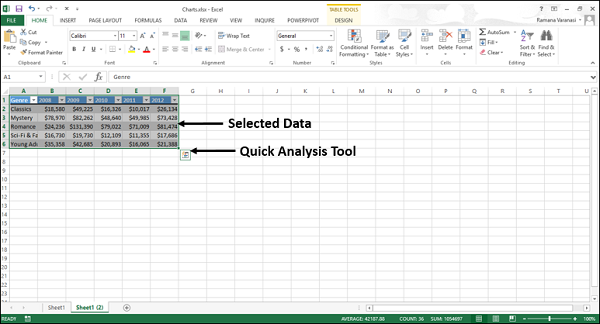
Step 2 − Click the Quick Analysis icon.

The Quick Analysis toolbar appears with the options FORMATTING, CHARTS, TOTALS, TABLES, SPARKLINES.

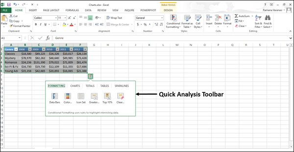
Step 3 − Click the CHARTS option.

Recommended Charts for your data will be displayed.

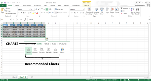
Step 4 − Point the mouse over the Recommended Charts. Previews of the available charts will be shown.

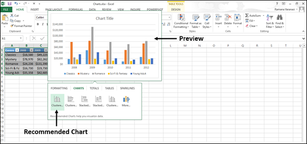
Step 5 − Click More.

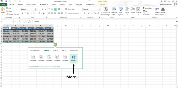
More Recommended Charts will be displayed.

Step 6 − Select the type of chart you like, click OK. The chart will be displayed in your worksheet.

Step 7 − Give a meaningful title to the chart by editing Chart Title.