Compare two columns for matches and differences in Excel

The task of comparing columns in Excel is one that will eventually be required of each and every one of us. When comparing and matching data in Microsoft Excel, you may do so in a variety of ways; however, the vast majority of these approaches focus on searching within a single column.

When you compare and match data in Microsoft Excel, you can do so in a variety of ways. Comparing the data in two columns in a large Excel spreadsheet can be a time-consuming process when working with such a document. You can save time by using Excel's functions to streamline the process, as compared to analyzing the columns and entering "Match" or "Mismatch" into a separate column in the spreadsheet.

In this tutorial you are going to learn some methods to compare two columns and find out matched data and mismatched data.

Compare Two Columns for Row Match using IF formula

If you want to receive a result that is more descriptive, you may use a straightforward IF formula that will return the word "Match" when the names are the same and the word "Mismatch" when the names are not the same. Let’s Understand through an example step by step.

Step 1

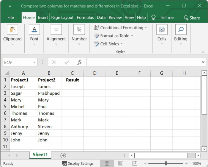
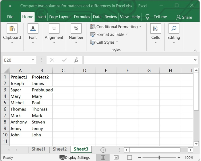
We have the names of employees who are working on Project1 and Project2, listed here in our Excel sheet. Some of the employees are tasked with contributing to both of the projects.

Step 2

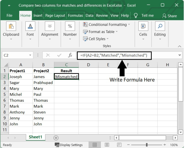
Select a blank cell from another column in which you want to get the result. In our case we have created another column named result and we are selecting C2 cell. Then type the following formula.

IF(A2=B2,"Matched","Mismatched") 

After adding the formula, when you press enter, it will compare the value of A2 cell with B2 cell and if they are equal, it will return "Matched", else "Mismatched".

Step 3

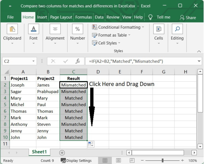
To get the result in remaining cells, click the ‘+’ sign that appears at the lower right corner of the cell C2, which activates the autofill function and then drag down. See the following image.

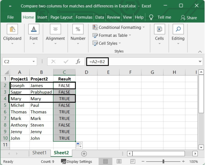
Note that we can use another formula here, that is =A2=B2. If there will be a match, it will return the result as True and False otherwise. See the below given image.

Using Conditional Formatting

Using the conditional formatting feature of Excel, it is possible to compare two columns and highlight the Unique and Duplicate cells between them.

Step 1

We have the names of employees who are working on Project1 and Project2, listed here in our Excel sheet. Some of the employees are tasked with contributing to both of the projects.

Select the data in the columns to whom you want to compare. In our case, we are selecting the data from cell A2 to B10.

Step 2

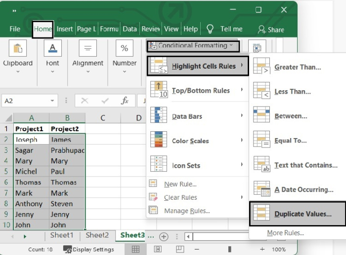
Now from the Ribbon, Go to Home Tab, then from the Styles group, select Conditional Formatting option. Then from the dropdown list, put cursor on Highlight Cell Rules, then go to Duplicate Values. (Home > Conditional Formatting > Highlight Cell Rules > Duplicate Values).

Step 3

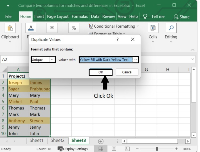
Now a popup window will appear. From the popup window, Duplicate if you want to Highlight the duplicate data, otherwise select unique. In the place of values with, select a colour combination from the dropdown list appears as per your choice.

In our case, we are selecting Unique to highlight the duplicate data and values with as Yellow Fill with Dark Yellow Text. Then click on OK.

Step 4

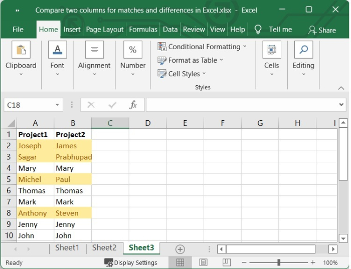
After clicking OK, we can see the unique values has been highlighted.

Conclusion

In this tutorial, we explained how you can use Excel's column comparison tool to look for matches (duplicates) and differences (unique values) in data.