
Article Categories
- All Categories
-
 Data Structure
-
 Networking
-
 RDBMS
RDBMS
-
 Operating System
-
 Java
Java
-
 MS Excel
-
 iOS
iOS
-
 HTML
HTML
-
 CSS
CSS
-
 Android
-
 Python
-
 C Programming
-
 C++
C++
-
 C#
C#
-
 MongoDB
-
 MySQL
MySQL
-
 Javascript
-
 PHP
PHP
-
 Economics & Finance
How to Automatically Create Borders if a Cell has Contents in Excel?
When trying to apply a border to cells in Excel, it can be a time-consuming and difficult process. This problem can be solved by automatically adding borders to the cells. Borders are nothing but the outline of the cells. This tutorial will help you understand how we can automatically create borders if a cell has contents in Excel.
Automatically Create Borders If a Cell Has Contents
Here we will use conditional formatting with a formula and select borders. Let us see an uncomplicated process to understand how we can automatically create borders if a cell has contents in Excel using conditional formatting.
Step 1
Consider an Excel sheet containing data similar to the data shown in the image below. We apply conditional formatting to the results.
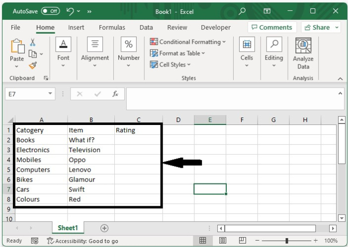
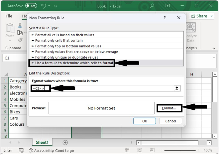
Now select the range in our case column c to which you want to apply borders, click on conditional formatting under "home," and select "new rule" to open formatting rules. Then click on "Use formula" and enter the formula as =C2< > and click on "Format" as shown in the below image.
In the formula, C2 represents where the formatting will start, and we change it based on our range of cells.
Step 2
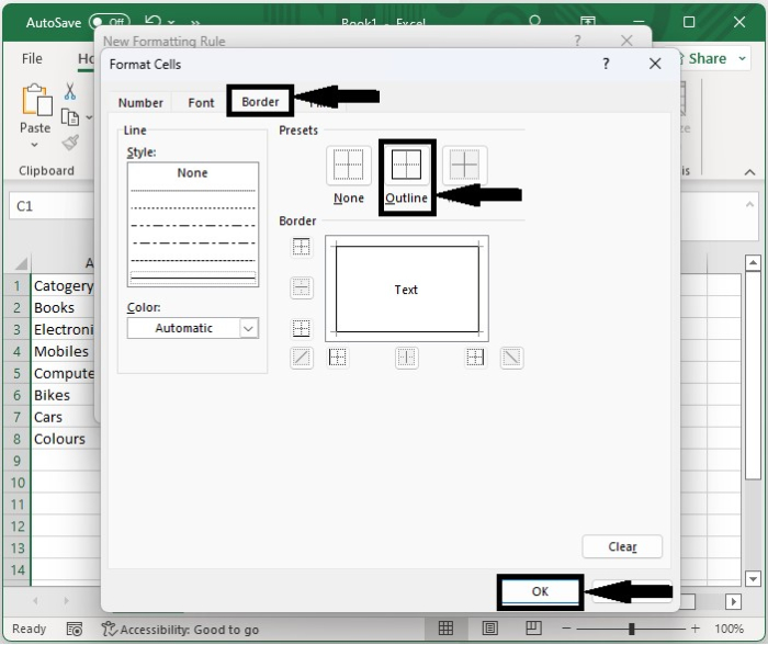
Now, as shown in the image below, click on "Border," then "Outline," then "OK," and then "OK" again to close the pop-up and complete our process.
Step 3
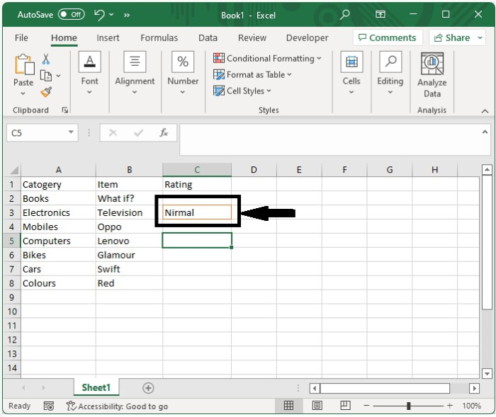
From now on, every time we enter the data in column C, the borders will be applied automatically. This process will only work for the newly added data; it will not work for the already existing data on the sheet.
Conclusion
In this tutorial, we used a simple example to demonstrate how we can automatically create borders if a cell has contents in Excel.

1K+ Views
