- Excel Power View - Home
- Overview
- Creation
- Sheet
- Visualizations
- Table Visualization
- Matrix Visualization
- Card Visualization
- Chart Visualizations
- Line Chart Visualization
- Bar Chart Visualization
- Column Chart Visualization
- Scatter & Bubble Chart Visualization
- Pie Chart Visualization
- Map Visualization
- Multiple Visualizations
- Tiles Visualizations
- Advanced Features
- Excel Power View and Data Model
- Hierarchies
- Key Performance Indicators
- Formatting a Report
- Sharing
Excel Power View and Data Model
Power View is based on the Data Model in your workbook that is created and managed by Power Pivot. You can access the Data Model from the Power Pivot window. Because of the optimization that Power Pivot uses in managing the Power Pivot window, you would be able to work with large data sets on the fly. Power View visualizations and their interactive features are possible because of the Data Model.
You can also create and/or modify the Data Model from the Power View sheet in your workbook.
For those readers for whom Data Model concepts in Excel are new, suggest to refer to Excel Power Pivot tutorial for the details. In this chapter, you will learn more about Power View and Data Model.
Power View and Data Model
You have learnt that Power View is based on the Data Model that is created and managed in Power Pivot window. You have also seen the Power of interactive visualizations that are based on large data such as Olympics data that is made part of the Data Model.
When you have a Data Model in your workbook, whenever you create a Power View sheet, it automatically gets the data tables from the Data Model along with the relationships defined among them, so that you can select fields from the related data tables.
If you have Excel tables in your workbook, you can link them to the data tables in the Data Model. However, if you have large data sets such as Olympics data, the Power View is optimized by directly creating the Data Model from the data source.
Once you have the Data Model in your workbook and relationships defined among the tables, you are all set to visualize and explore data in Power View.
You can refresh the data in the Data Model to update the modifications made in the data sources from where you have created the Data Model.
Creating Data Model from Power View Sheet
You can also create the Data Model directly from the Power View sheet as follows −
Start with a new workbook that contains Salesperson data and Sales data in two worksheets.
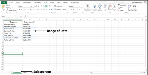
Create a table from the range of data in the Salesperson worksheet and name it Salesperson.
Create a table from the range of data in the Sales worksheet and name it Sales.
You have two tables Salesperson and Sales in your workbook.
Click the Sales table in the Sales worksheet.
Click the INSERT tab on the Ribbon.
Click Power View in the Reports group.
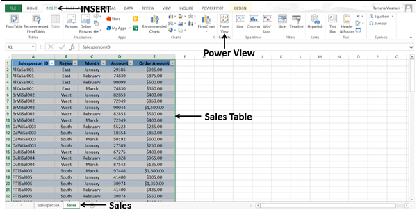
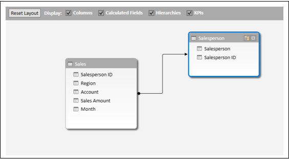
A new Power View sheet will be created in your workbook. A Table visualization appears with all the fields in the Sales table. Note that you do not have a Data Model in your workbook.
As you can observe in the Power View Fields list, both the tables that are in the workbook are displayed. However, in the Power View only the active table (Sales) fields are displayed.
In the Table in the Power View, Salesperson ID is displayed. Suppose you want to display the Salesperson name instead.
In the Power View Fields list, make the following changes −
- Deselect the field Salesperson ID in the Sales table.
- Select the field Salesperson in the Salesperson table.
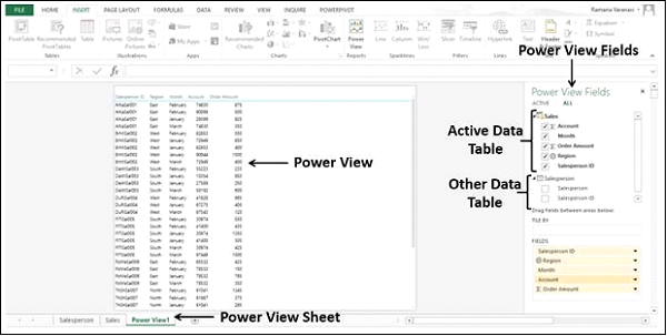
As you do not have a Data Model in the workbook, no relationship exists between the two tables. No data is displayed in Power View. Excel displays messages directing you what to do.
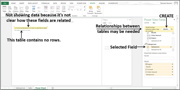
A CREATE button will be displayed in the Power View Fields pane. Click the CREATE button.
A Create Relationship dialog box appears in the Power View Sheet itself.
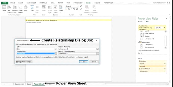
Create a relationship between the two tables using the Salesperson ID field.
Without closing the Power View sheet, you have successfully created the following −
- The Data Model with the two tables, and
- The relationship between the two tables.
The field Salesperson appears in the Table in Power View along with the Sales data.
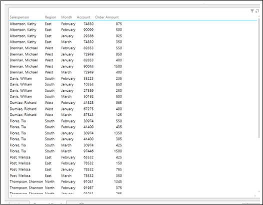
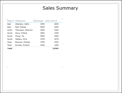
Rearrange the fields in the FIELDS area to Region, Salesperson and Order Amount in that order.
Drag the field Month to the area TILE BY.
Switch visualization to Matrix.
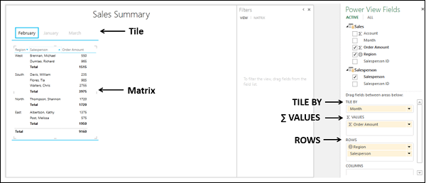
You can see that for each of the Regions, the Salespersons of that Region and sum of Order Amount are displayed. Subtotals are displayed for each Region. The display is month-wise as selected in the Tiles. When you select a Month in the Tiles, the data of that Month will be displayed in the Matrix.
You are able to work with the Power View visualizations as the Data Model is now created. You can check it in the Power Pivot window.
Click the POWERPIVOT tab on the Ribbon.
Click Manage in the Data Model group. The Power Pivot window appears.
The data tables Salesperson and Sales are created in the Data Model along with the defined relationship.
Modifying Data Model from Power View Sheet
You can also modify the Data Model in your workbook from the Power View sheet by adding data tables and creating relationships among the data tables.
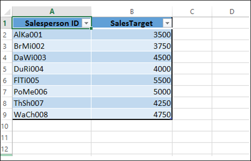
- Consider the Excel table SalesTarget in your workbook.
Click on the Power View sheet.
Click on the Matrix.
Switch visualization to Table.
Deselect the field Month.
Click the ALL tab in the Power View Fields pane. You can see that the table SalesTarget is included.
Click the POWERPIVOT tab on the Ribbon.
Click Manage. The Power Pivot window appears displaying the Data Model.
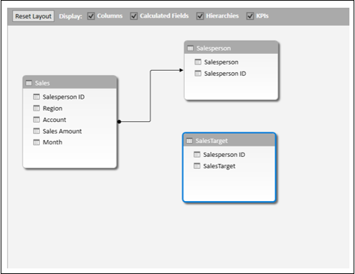
You can add a data table to the Data Model from Power View itself.
Click on the Power View sheet.
Select the field SalesTarget in the SalesTarget table in the Power View Fields list.
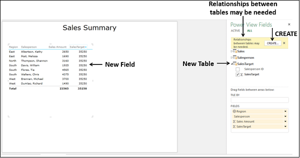
The new field SalesTarget is added to the table, but a message saying Relationships between tables may be needed. A CREATE button appears.
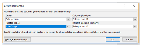
Click the CREATE button. The Create Relationship dialog box appears.
Create a relationship with the SalesPersonID field and click OK.
Click in the Power Pivot window.
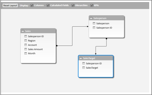
The relationship you have created in the Power View sheet is reflected in the Data Model.
Click the arrow in the field SalesTarget in the FIELDS area in the Power View Fields pane.
Select Do Not Summarize from the dropdown list.
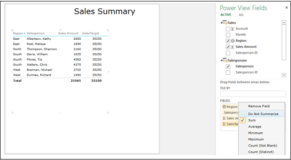
Rearrange the fields in the Fields area.