- Digital Communication - Home
- Analog to Digital
- Pulse Code Modulation
- Sampling
- Quantization
- Differential PCM
- Delta Modulation
- Techniques
- Line Codes
- Data Encoding Techniques
- Pulse Shaping
- Digital Modulation Techniques
- Amplitude Shift Keying
- Frequency Shift Keying
- Phase Shift Keying
- Quadrature Phase Shift Keying
- Differential Phase Shift Keying
- M-ary Encoding
- Information Theory
- Source Coding Theorem
- Channel Coding Theorem
- Error Control Coding
- Spread Spectrum Modulation
Digital Communication - Line Codes
A line code is the code used for data transmission of a digital signal over a transmission line. This process of coding is chosen so as to avoid overlap and distortion of signal such as inter-symbol interference.
Properties of Line Coding
Following are the properties of line coding −
As the coding is done to make more bits transmit on a single signal, the bandwidth used is much reduced.
For a given bandwidth, the power is efficiently used.
The probability of error is much reduced.
Error detection is done and the bipolar too has a correction capability.
Power density is much favorable.
The timing content is adequate.
Long strings of 1s and 0s is avoided to maintain transparency.
Types of Line Coding
There are 3 types of Line Coding
- Unipolar
- Polar
- Bi-polar
Unipolar Signaling
Unipolar signaling is also called as On-Off Keying or simply OOK.
The presence of pulse represents a 1 and the absence of pulse represents a 0.
There are two variations in Unipolar signaling −
- Non Return to Zero (NRZ)
- Return to Zero (RZ)
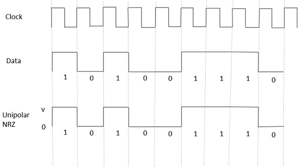
Unipolar Non-Return to Zero (NRZ)
In this type of unipolar signaling, a High in data is represented by a positive pulse called as Mark, which has a duration T0 equal to the symbol bit duration. A Low in data input has no pulse.
The following figure clearly depicts this.
Advantages
The advantages of Unipolar NRZ are −
- It is simple.
- A lesser bandwidth is required.
Disadvantages
The disadvantages of Unipolar NRZ are −
No error correction done.
Presence of low frequency components may cause the signal droop.
No clock is present.
Loss of synchronization is likely to occur (especially for long strings of 1s and 0s).
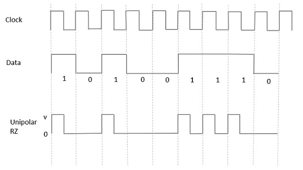
Unipolar Return to Zero (RZ)
In this type of unipolar signaling, a High in data, though represented by a Mark pulse, its duration T0 is less than the symbol bit duration. Half of the bit duration remains high but it immediately returns to zero and shows the absence of pulse during the remaining half of the bit duration.
It is clearly understood with the help of the following figure.
Advantages
The advantages of Unipolar RZ are −
- It is simple.
- The spectral line present at the symbol rate can be used as a clock.
Disadvantages
The disadvantages of Unipolar RZ are −
- No error correction.
- Occupies twice the bandwidth as unipolar NRZ.
- The signal droop is caused at the places where signal is non-zero at 0 Hz.
Polar Signaling
There are two methods of Polar Signaling. They are −
- Polar NRZ
- Polar RZ
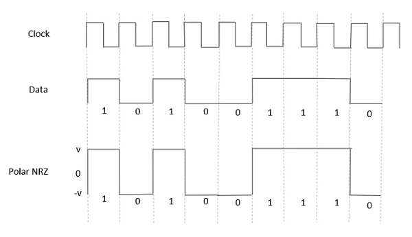
Polar NRZ
In this type of Polar signaling, a High in data is represented by a positive pulse, while a Low in data is represented by a negative pulse. The following figure depicts this well.
Advantages
The advantages of Polar NRZ are −
- It is simple.
- No low-frequency components are present.
Disadvantages
The disadvantages of Polar NRZ are −
No error correction.
No clock is present.
The signal droop is caused at the places where the signal is non-zero at 0 Hz.
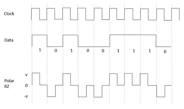
Polar RZ
In this type of Polar signaling, a High in data, though represented by a Mark pulse, its duration T0 is less than the symbol bit duration. Half of the bit duration remains high but it immediately returns to zero and shows the absence of pulse during the remaining half of the bit duration.
However, for a Low input, a negative pulse represents the data, and the zero level remains same for the other half of the bit duration. The following figure depicts this clearly.
Advantages
The advantages of Polar RZ are −
- It is simple.
- No low-frequency components are present.
Disadvantages
The disadvantages of Polar RZ are −
No error correction.
No clock is present.
Occupies twice the bandwidth of Polar NRZ.
The signal droop is caused at places where the signal is non-zero at 0 Hz.
Bipolar Signaling
This is an encoding technique which has three voltage levels namely +, - and 0. Such a signal is called as duo-binary signal.
An example of this type is Alternate Mark Inversion (AMI). For a 1, the voltage level gets a transition from + to or from to +, having alternate 1s to be of equal polarity. A 0 will have a zero voltage level.
Even in this method, we have two types.
- Bipolar NRZ
- Bipolar RZ
From the models so far discussed, we have learnt the difference between NRZ and RZ. It just goes in the same way here too. The following figure clearly depicts this.
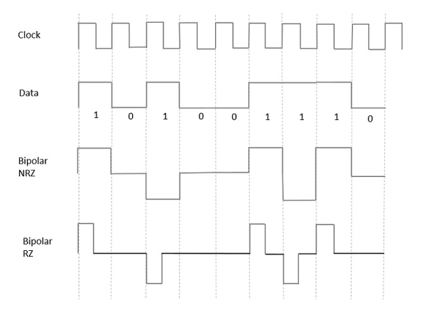
The above figure has both the Bipolar NRZ and RZ waveforms. The pulse duration and symbol bit duration are equal in NRZ type, while the pulse duration is half of the symbol bit duration in RZ type.
Advantages
Following are the advantages −
It is simple.
No low-frequency components are present.
Occupies low bandwidth than unipolar and polar NRZ schemes.
This technique is suitable for transmission over AC coupled lines, as signal drooping doesnt occur here.
A single error detection capability is present in this.
Disadvantages
Following are the disadvantages −
- No clock is present.
- Long strings of data causes loss of synchronization.
Power Spectral Density
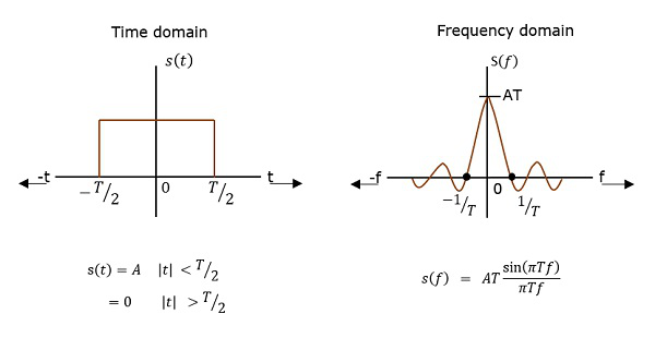
The function which describes how the power of a signal got distributed at various frequencies, in the frequency domain is called as Power Spectral Density (PSD).
PSD is the Fourier Transform of Auto-Correlation (Similarity between observations). It is in the form of a rectangular pulse.
PSD Derivation
According to the Einstein-Wiener-Khintchine theorem, if the auto correlation function or power spectral density of a random process is known, the other can be found exactly.
Hence, to derive the power spectral density, we shall use the time auto-correlation $(R_x(\tau))$ of a power signal $x(t)$ as shown below.
$R_x(\tau) = \lim_{T_p \rightarrow \infty}\frac{1}{T_p}\int_{\frac{{-T_p}}{2}}^{\frac{T_p}{2}}x(t)x(t + \tau)dt$
Since $x(t)$ consists of impulses, $R_x(\tau)$ can be written as
$R_x(\tau) = \frac{1}{T}\displaystyle\sum\limits_{n = -\infty}^\infty R_n\delta(\tau - nT)$
Where $R_n = \lim_{N \rightarrow \infty}\frac{1}{N}\sum_ka_ka_{k + n}$
Getting to know that $R_n = R_{-n}$ for real signals, we have
$S_x(w) = \frac{1}{T}(R_0 + 2\displaystyle\sum\limits_{n = 1}^\infty R_n \cos nwT)$
Since the pulse filter has the spectrum of $(w) \leftrightarrow f(t)$, we have
$s_y(w) = \mid F(w) \mid^2S_x(w)$
$= \frac{\mid F(w) \mid^2}{T}(\displaystyle\sum\limits_{n = -\infty}^\infty R_ne^{-jnwT_{b}})$
$= \frac{\mid F(w) \mid^2}{T}(R_0 + 2\displaystyle\sum\limits_{n = 1}^\infty R_n \cos nwT)$
Hence, we get the equation for Power Spectral Density. Using this, we can find the PSD of various line codes.