- Digital Communication - Home
- Analog to Digital
- Pulse Code Modulation
- Sampling
- Quantization
- Differential PCM
- Delta Modulation
- Techniques
- Line Codes
- Data Encoding Techniques
- Pulse Shaping
- Digital Modulation Techniques
- Amplitude Shift Keying
- Frequency Shift Keying
- Phase Shift Keying
- Quadrature Phase Shift Keying
- Differential Phase Shift Keying
- M-ary Encoding
- Information Theory
- Source Coding Theorem
- Channel Coding Theorem
- Error Control Coding
- Spread Spectrum Modulation
Digital Communication - Delta Modulation
The sampling rate of a signal should be higher than the Nyquist rate, to achieve better sampling. If this sampling interval in Differential PCM is reduced considerably, the sampleto-sample amplitude difference is very small, as if the difference is 1-bit quantization, then the step-size will be very small i.e., Δ (delta).
Delta Modulation
The type of modulation, where the sampling rate is much higher and in which the stepsize after quantization is of a smaller value Δ, such a modulation is termed as delta modulation.
Features of Delta Modulation
Following are some of the features of delta modulation.
An over-sampled input is taken to make full use of the signal correlation.
The quantization design is simple.
The input sequence is much higher than the Nyquist rate.
The quality is moderate.
The design of the modulator and the demodulator is simple.
The stair-case approximation of output waveform.
The step-size is very small, i.e., Δ (delta).
The bit rate can be decided by the user.
This involves simpler implementation.
Delta Modulation is a simplified form of DPCM technique, also viewed as 1-bit DPCM scheme. As the sampling interval is reduced, the signal correlation will be higher.
Delta Modulator
The Delta Modulator comprises of a 1-bit quantizer and a delay circuit along with two summer circuits. Following is the block diagram of a delta modulator.
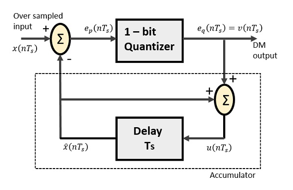
The predictor circuit in DPCM is replaced by a simple delay circuit in DM.
From the above diagram, we have the notations as −
$x(nT_{s})$ = over sampled input
$e_{p}(nT_{s})$ = summer output and quantizer input
$e_{q}(nT_{s})$ = quantizer output = $v(nT_s)$
$\widehat{x}(nT_{s})$ = output of delay circuit
$u(nT_{s})$ = input of delay circuit
Using these notations, now we shall try to figure out the process of delta modulation.
$e_{p}(nT_{s}) = x(nT_{s}) - \widehat{x}(nT_{s})$
---------equation 1
$= x(nT_{s}) - u([n - 1]T_{s})$
$= x(nT_{s}) - [\widehat{x} [[n - 1]T_{s}] + v[[n-1]T_{s}]]$
---------equation 2
Further,
$v(nT_{s}) = e_{q}(nT_{s}) = S.sig.[e_{p}(nT_{s})]$
---------equation 3
$u(nT_{s}) = \widehat{x}(nT_{s})+e_{q}(nT_{s})$
Where,
$\widehat{x}(nT_{s})$ = the previous value of the delay circuit
$e_{q}(nT_{s})$ = quantizer output = $v(nT_s)$
Hence,
$u(nT_{s}) = u([n-1]T_{s}) + v(nT_{s})$
---------equation 4
Which means,
The present input of the delay unit
= (The previous output of the delay unit) + (the present quantizer output)
Assuming zero condition of Accumulation,
$u(nT_{s}) = S \displaystyle\sum\limits_{j=1}^n sig[e_{p}(jT_{s})]$
Accumulated version of DM output = $\displaystyle\sum\limits_{j = 1}^n v(jT_{s})$
---------equation 5
Now, note that
$\widehat{x}(nT_{s}) = u([n-1]T_{s})$
$= \displaystyle\sum\limits_{j = 1}^{n - 1} v(jT_{s})$
---------equation 6
Delay unit output is an Accumulator output lagging by one sample.
From equations 5 & 6, we get a possible structure for the demodulator.
A Stair-case approximated waveform will be the output of the delta modulator with the step-size as delta (Δ). The output quality of the waveform is moderate.
Delta Demodulator
The delta demodulator comprises of a low pass filter, a summer, and a delay circuit. The predictor circuit is eliminated here and hence no assumed input is given to the demodulator.
Following is the diagram for delta demodulator.
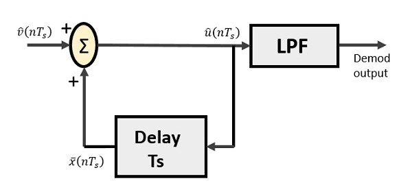
From the above diagram, we have the notations as −
$\widehat{v}(nT_{s})$ is the input sample
$\widehat{u}(nT_{s})$ is the summer output
$\bar{x}(nT_{s})$ is the delayed output
A binary sequence will be given as an input to the demodulator. The stair-case approximated output is given to the LPF.
Low pass filter is used for many reasons, but the prominent reason is noise elimination for out-of-band signals. The step-size error that may occur at the transmitter is called granular noise, which is eliminated here. If there is no noise present, then the modulator output equals the demodulator input.
Advantages of DM Over DPCM
1-bit quantizer
Very easy design of the modulator and the demodulator
However, there exists some noise in DM.
Slope Over load distortion (when Δ is small)
Granular noise (when Δ is large)
Adaptive Delta Modulation (ADM)
In digital modulation, we have come across certain problem of determining the step-size, which influences the quality of the output wave.
A larger step-size is needed in the steep slope of modulating signal and a smaller stepsize is needed where the message has a small slope. The minute details get missed in the process. So, it would be better if we can control the adjustment of step-size, according to our requirement in order to obtain the sampling in a desired fashion. This is the concept of Adaptive Delta Modulation.
Following is the block diagram of Adaptive delta modulator.
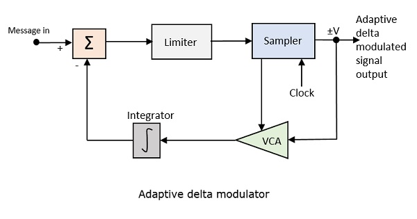
The gain of the voltage controlled amplifier is adjusted by the output signal from the sampler. The amplifier gain determines the step-size and both are proportional.
ADM quantizes the difference between the value of the current sample and the predicted value of the next sample. It uses a variable step height to predict the next values, for the faithful reproduction of the fast varying values.
